Week 1: Channel flow simulation using CONVERGE CFD
AIM
We have to perform Channel flow simulation using CONVERGE CFD and get results of Plots for velocity, pressure, mass flow rate, and total cell count for different mesh size as:-
dx = 2e-4m, dy = 2e-4m, dz = 2e-4m
dx = 1.5e-4m, dy = 1.5e-4m, dz = 1.5e-4m
dx = 1.0e-4m, dy = 1.0e-4m, dz = 1.0e-4m
INTRODUCTION/THEORY
In fluid dynamics, internal flow is a flow for which the fluid is confined by a surface. Detailed knowledge of behaviour of internal flow regimes is of importance in engineering, because circular pipes can withstand high pressures and hence are used to convey liquids. Non-circular ducts are used to transport low-pressure gases, such as air in cooling and heating systems. The internal flow configuration is a convenient geometry for heating and cooling fluids used in energy conversion technologies.
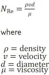
The Reynolds number is the ratio of inertial forces to viscous forces. The Reynolds number is a dimensionless number used to categorize the fluids systems in which the effect of viscosity is important in controlling the velocities or the flow pattern of a fluid. Mathematically, the Reynolds number, NRe, is defined as
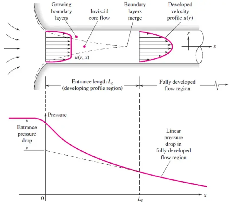
In fluid mechanics, pipe flow is a type of liquid flow within a closed conduit, such as a pipe or tube. The other type of flow within a conduit is open channel flow. These two types of flow are similar in many ways, but differ in one important aspect. Pipe flow does not have a free surface which is found in open-channel flow. Pipe flow, being confined within closed conduit, does not exert direct atmospheric pressure, but does exert hydraulic pressure on the conduit.
The flow regime (laminar or transition or turbulent) of internal flows is primarily a function of the Reynolds number (inertial force/viscous force).In pipes, Reynolds number below 2000 is laminar, between 2000 and 4000 is transition flow, above 4000 is turbulent flow.
In pipe flow, the pressure gradient along the pipe is the main driving force.
One important concept in pipe flows, is that of the boundary layer. A boundary layer is the layer of fluid in the immediate vicinity of a bounding surface where the effects of viscosity are significant.
GEOMETRY
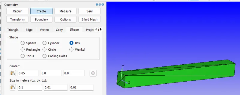
We will design the channel by defining the centre and size.
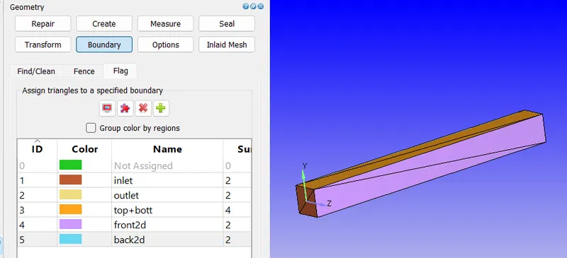
Name the wall and boundaries
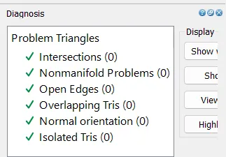
Diagnose the geometry for any errors
CASE SETUP
Our goal will be to describe all the following parameters for our setup:-
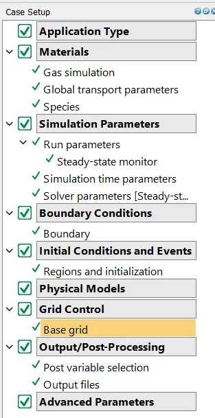
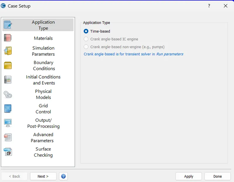
Step 1) Define the application
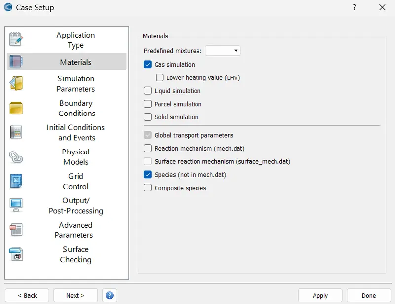
Step 2) Describe the material and phase parameter
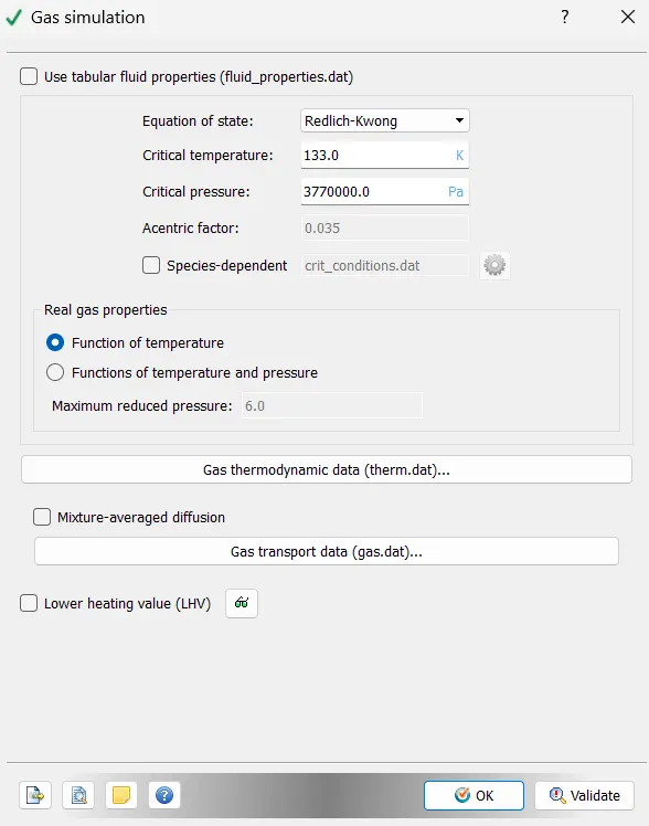
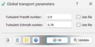

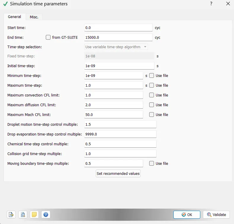
Step 3) Describe the simulation para.
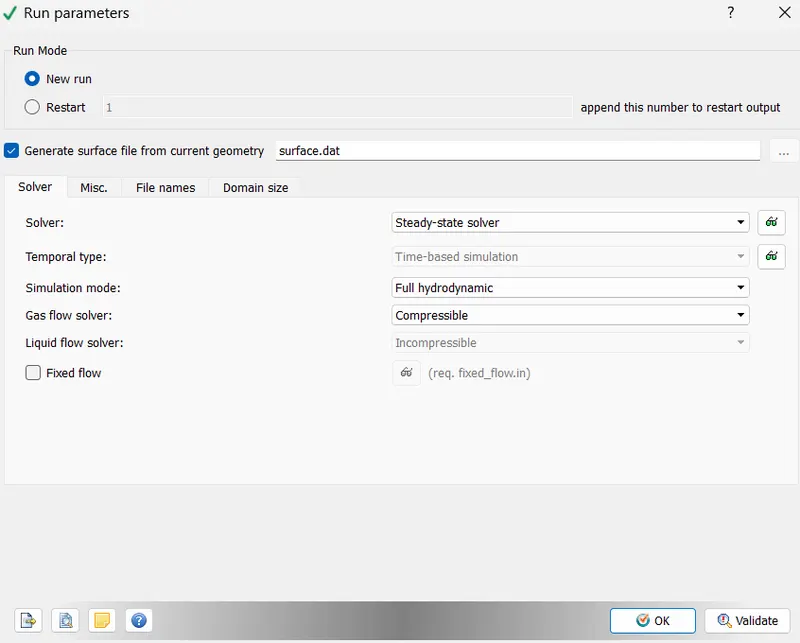
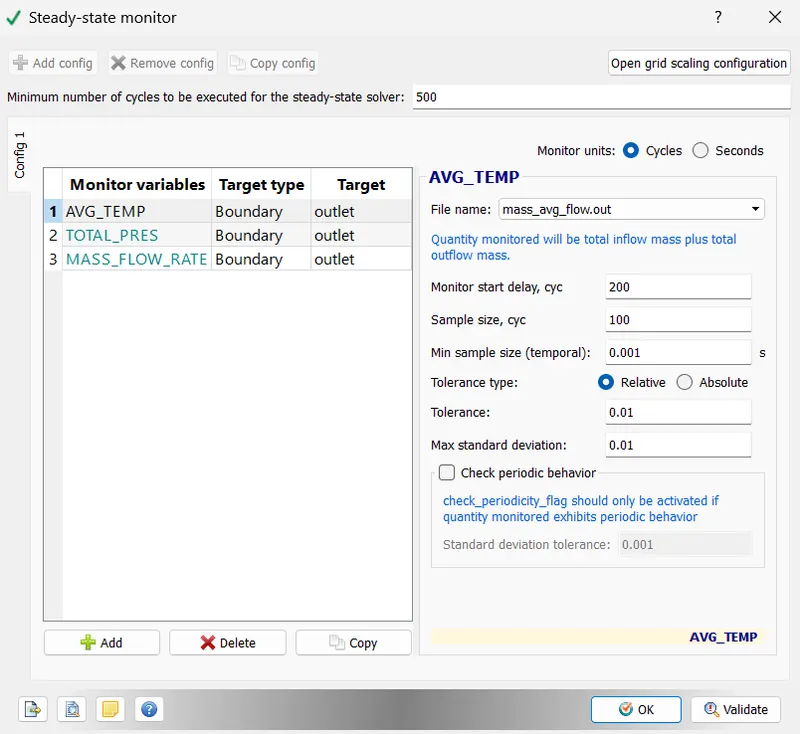
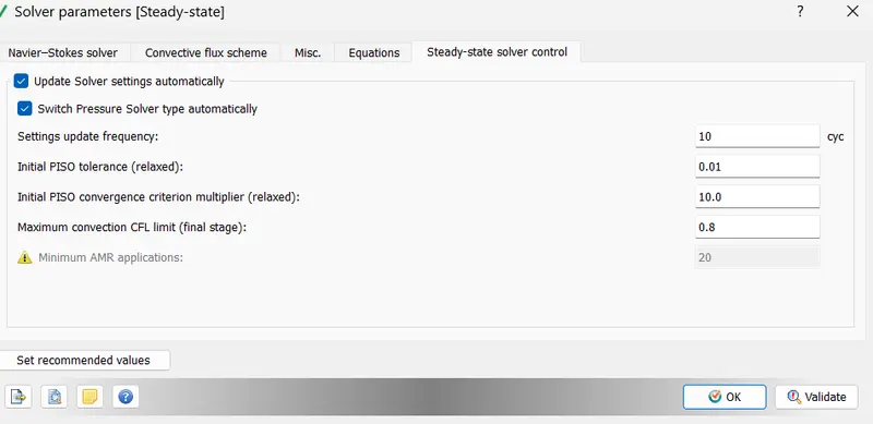
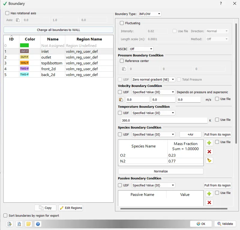
Step 4) Define boundary and it's conditions
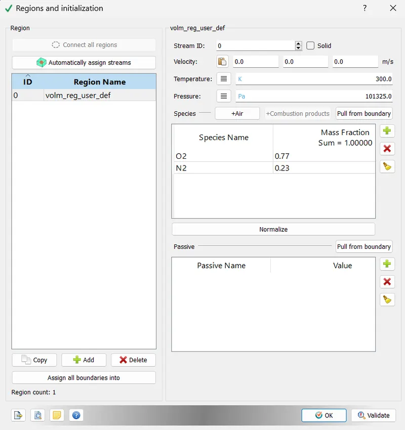
Step 5) State the initial condition
Step 6) Make sure we are using the steady model
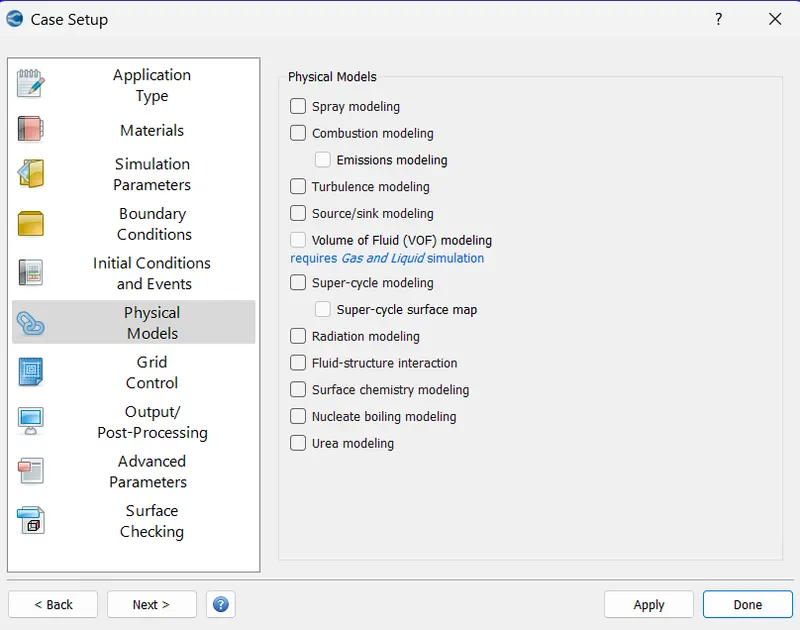
Step 7) Define the mesh grid size for differnt cases
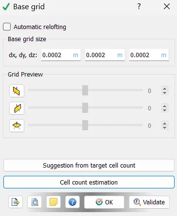
Step 8) Define the vaariables to be monitersed in our simulation
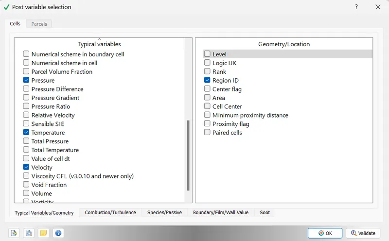
1. Post variable selection - Pressure, Temperature, Velocity
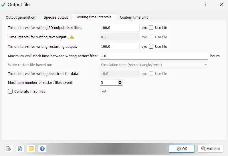
2. Output files -
The time interval for writing 3D output data files: 100
The time interval for writing restarting output: 100
Maximum restart files saved: 3
Step 9) Export the setup files to a new folder

RESULTS
Case 1: Mesh => dx = 2e-4m, dy = 2e-4m, dz = 2e-4m
1. Velocity plot:
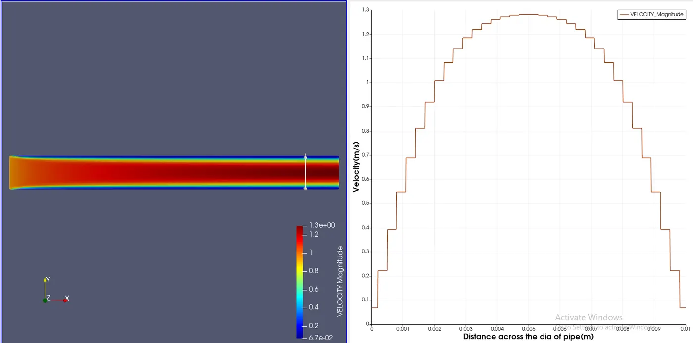
Velocity plot on a vertical line at x=0.09m (near the exit of the channel). The peak velocity near the center of the channel is 1.28159 m/s. The plot values adhere to the principle of boundary layer theory by giving us the parabolic nature as expected.
2. Pressure plot:
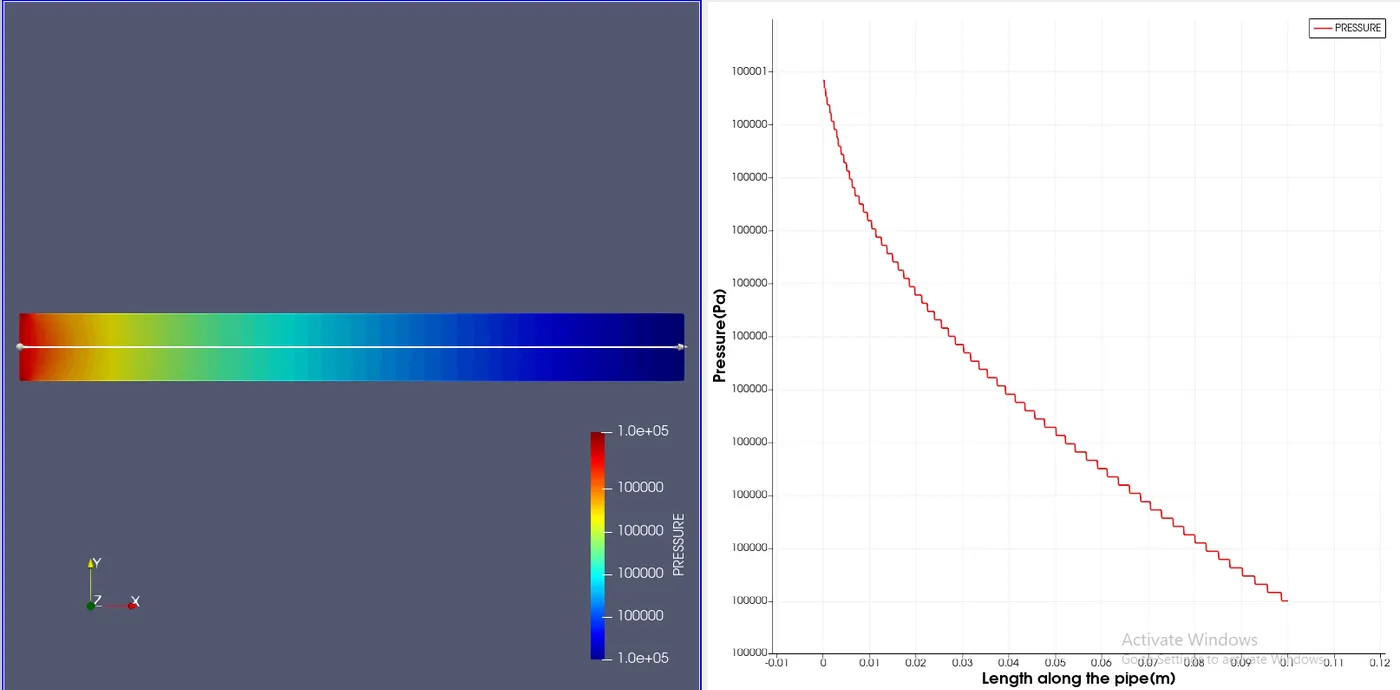
The pressure is constantly decreasing along the pipe as expected according to the boundary conditions given.
3. Mass flow rate:
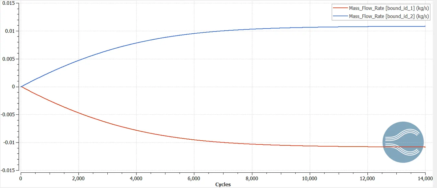
The mass flow rate is -0.0108252 m/s for the inlet and 0.0108251 m/s for the outlet. (The sign indicates if the flow is inside the channel or outside the channel)
4. Cell count:
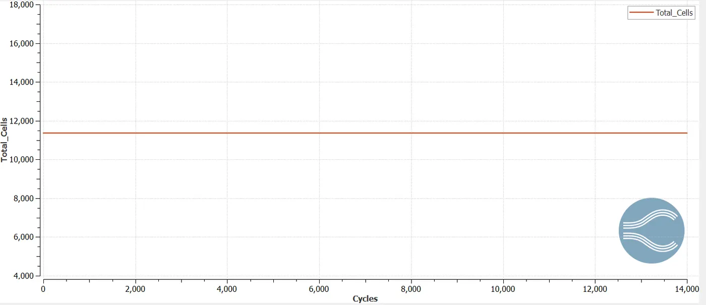
The cell count for the first mesh is 11,356 which required only 1 processor for solving.
Case 2: Mesh => dx = 1.5e-4m, dy = 1.5e-4m, dz = 1.5e-4m
1. Velocity plot :
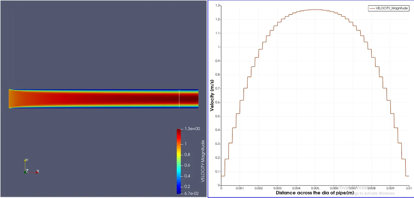
Velocity plot on a vertical line at x=0.09m (near the exit of the channel). The peak velocity near the center of the channel is 1.27049 m/s. The plot values adhere to the principle of boundary layer theory by resulting parabolic profile.
2. Pressure plot:
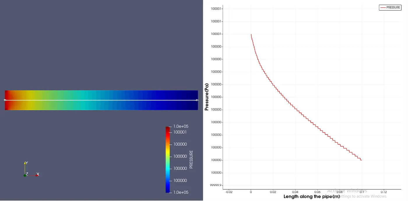
The pressure is constantly decreasing along the pipe as expected according to the boundary conditions given.
3. Mass flow rate:
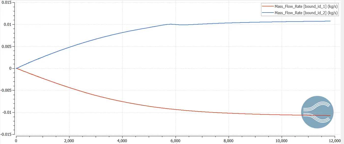
The mass flow rate is -0.0107176 m/s for the inlet and 0.0107124 m/s for the outlet, which is a bit less than what aquired in previous case. (The sign indicates if the flow is inside the channel or outside the channel)
4. Cell count:
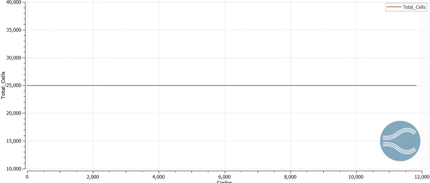
The cell count for the second mesh is 25,000.
Case 3: Mesh => dx = 1.0e-4m, dy = 1.0e-4m, dz = 1.0e-4m
1. Velocity plot:
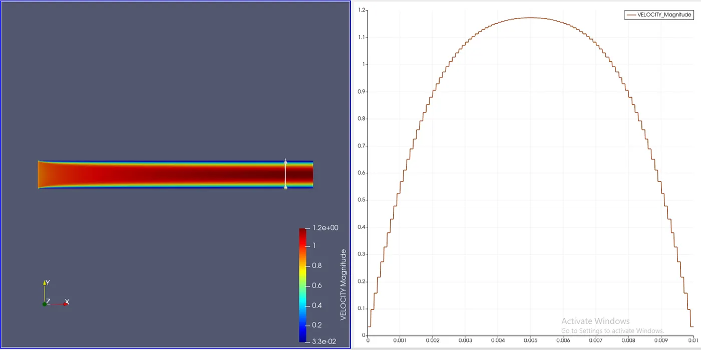
Velocity plot on a vertical line at x=0.09m (near the exit of the channel). The peak velocity near the center of the channel is 1.17224 m/s. The plot values adhere to the principle of boundary layer theory by giving parabolic profile.
2. Pressure plot:
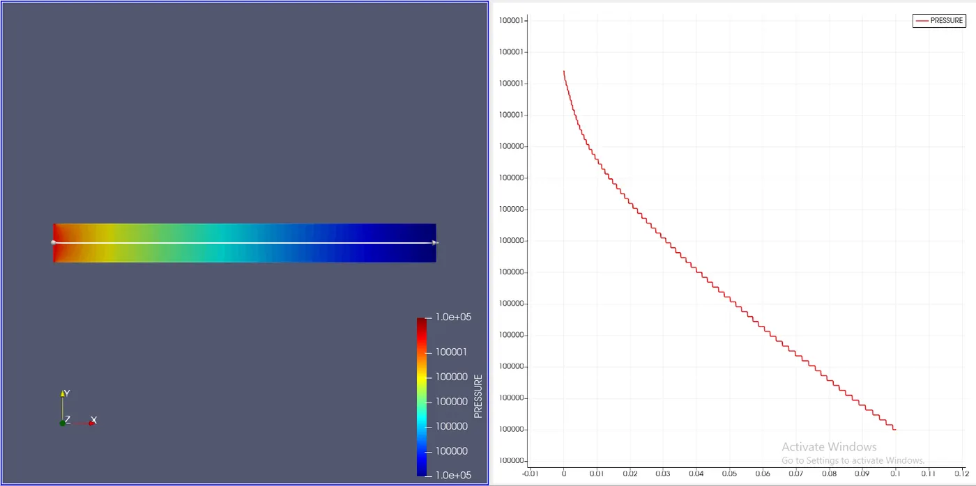
The pressure is constantly decreasing along the pipe as expected according to the boundary conditions given.
3. Mass flow rate:
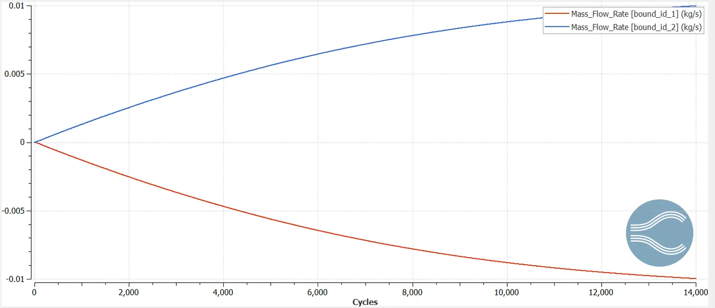
The mass flow rate is -0.00997052 m/s for the inlet and 0.00997051 m/s for the outlet, which is a bit less than what aquired in previous case. (The sign indicates if the flow is inside the channel or outside the channel)
4. Cell count:
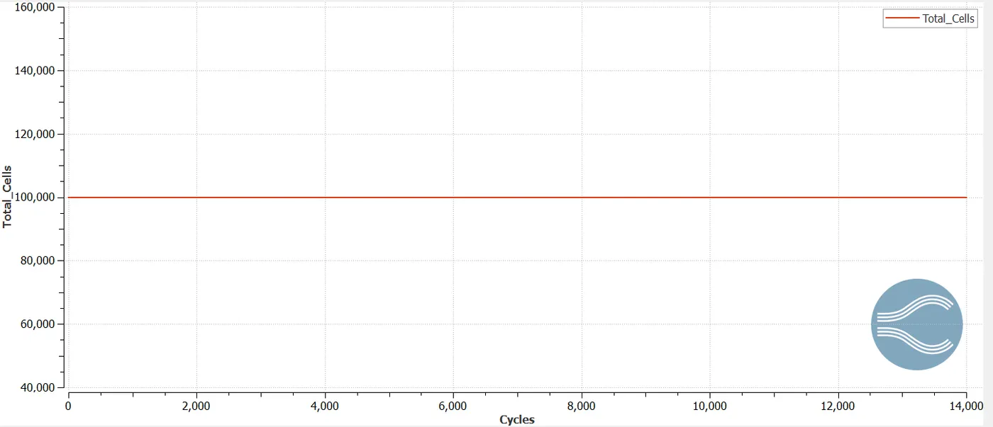
The cell count for the third mesh is 100,000.
ANIMATIONS
1) Velocity Amimation
The contour pattern of results for all 3 cases were almost same. Initially, throught it was blue, but as the iterations proceed we can observe profile regions turning red. Wall boundary regions were blue all the time justifying the no-slip condition we gave to the cylinder walls. Boudary layer effect gives us the parabolic profile clearly.
2) Pressure Profile
Slow decrease in pressure as the iterations proceed occurs. Initially, the region was red but with cycles it started turning blue gradually.
CONCLUSION
Following points can be concluded from our results:-
1. Pressure, driving force in our case keeps on decreasing which can be witnessed from pressure contours.
2. Velocity contours depict the formation of no-slip condition at the wall which results in the formation of parabolic shaped boundary layers.
3. The plots are in the form of steps because of the mesh size. The finer the mesh, smoother will be the curve.
4. The mass-flow rate plot achieved confirms the conservation of mass. The mass-flow rate value decreases by a very small amount as the mesh becomes finer or smaller.
5. Peak velocity value drops as the mesh becomes finer.