Week 1: Channel flow simulation using CONVERGE CFD
AIM:
To simulate the air through a channel for three different mesh sizes of (dx=dy=dz=2e-4,1.5e-4 and 1.2e-4) and to generate the flow and explain with aid of plots, animations of velocity, pressure and mass flow rate
DESCRIPTION:
The flow through a rectangular channel is characterized by 0 velocity at the wall due to no slip condition. Gradually as we move to the center of the channel in the vertical direction, the velocity magnitude increases and the maximum value is attained at the center. Thus resulting in parabolic profile.
In our simulation we assume that the flow across the duct is two dimensional, varying only in the X and Y direction. Flow across any cross section is assumed to be constant and no variation is considered along Z-direction.
CASE SETUP:
GEOMETRY CREATION:
Creating the rectangular box using the following create>box and giving the dimensions
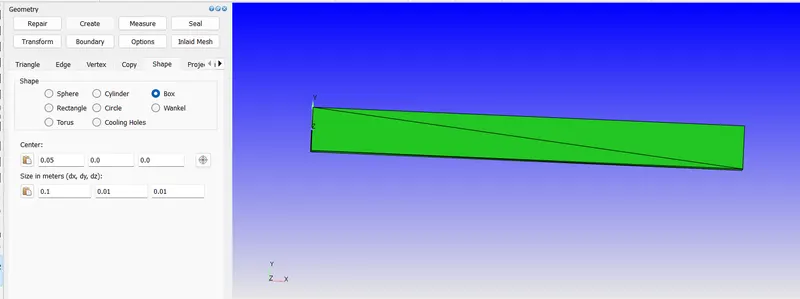
As we see many triangles in the model we combine them and create the boundary
BOUNDARY CREATION
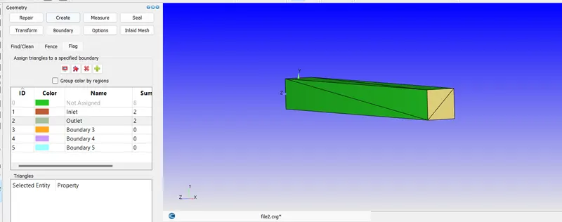
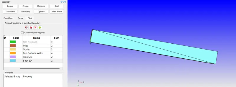
Using Boundary>Flag and add boundary we create the required boundaries
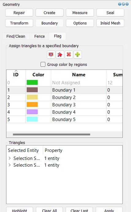
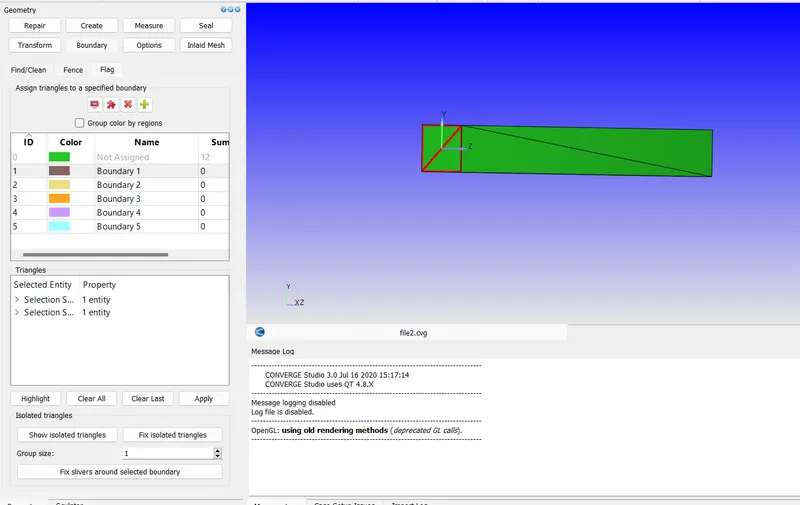
Then selecting boundary with ID number 1 and selecting the triangles and naming ID1 as inlet
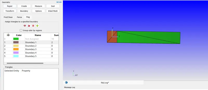
For outlet boundary
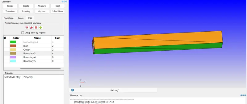
Applying top and bottom faces for boundary 3
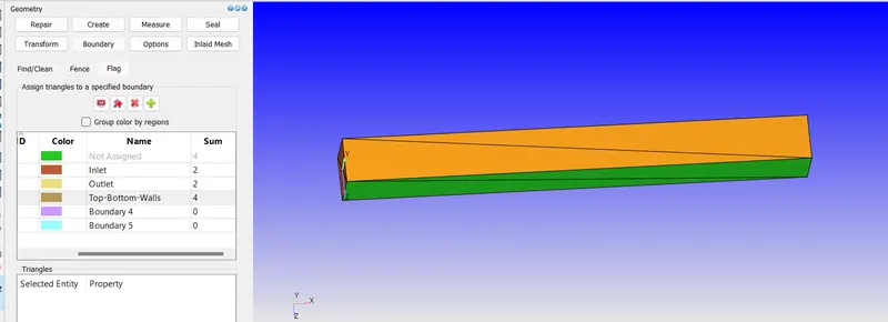
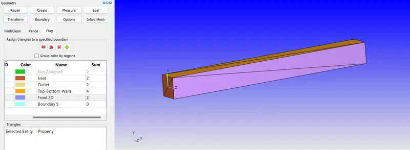
For other faces
Enabling the normals
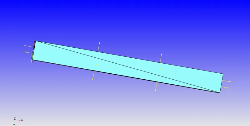
We see that as fluid flows inside the geometry Normals should even point inside
So now using Transform>Normal select any triangle and apply which cleans up the geometry as follows
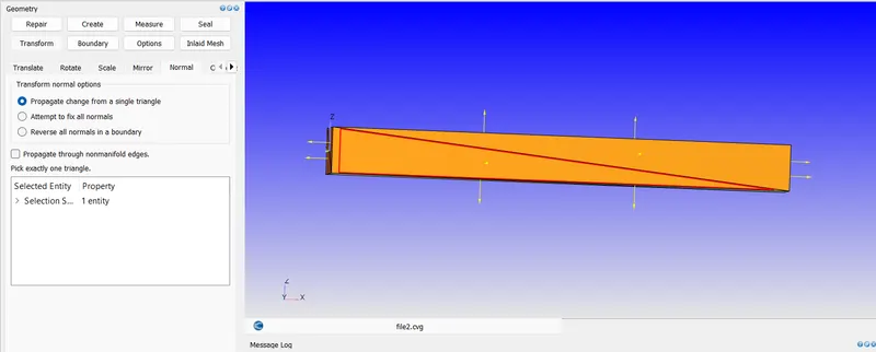
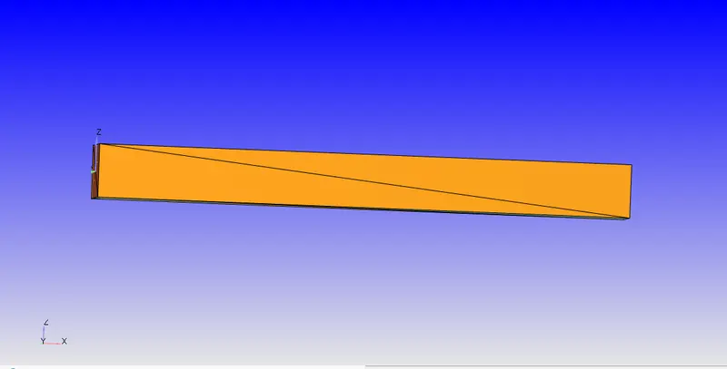
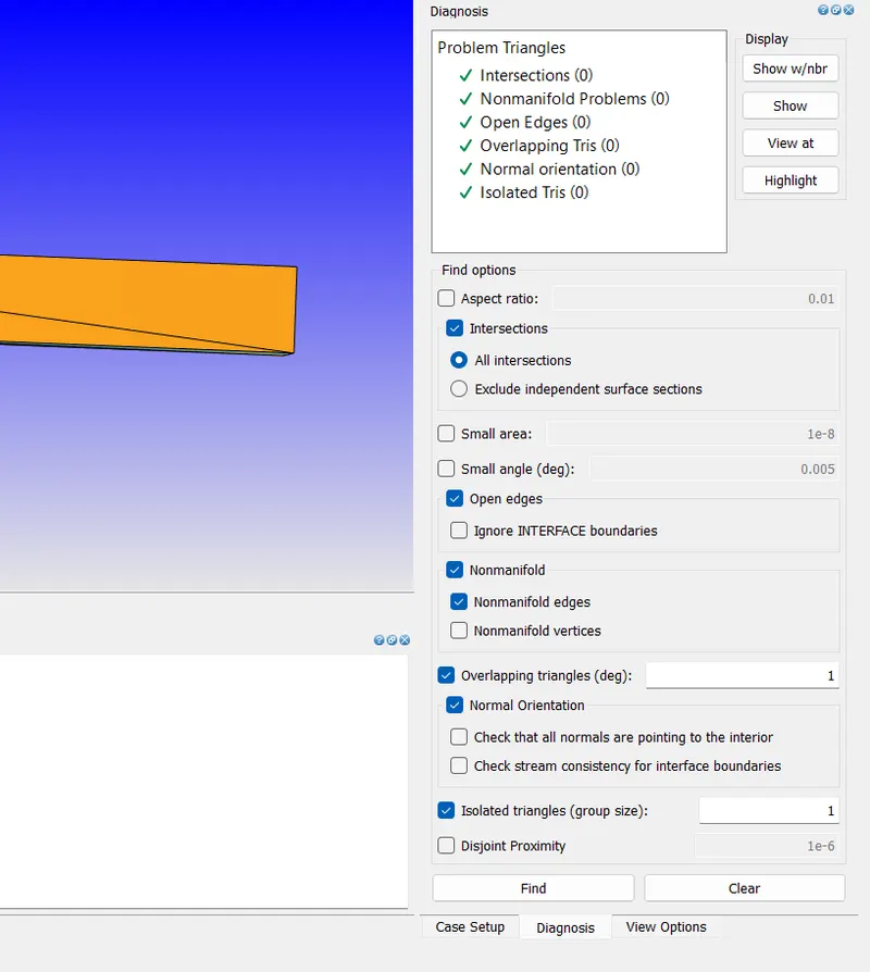
To confirm there are no errors go to bottom right corner for diagnosis and check for errors
So we see no errors
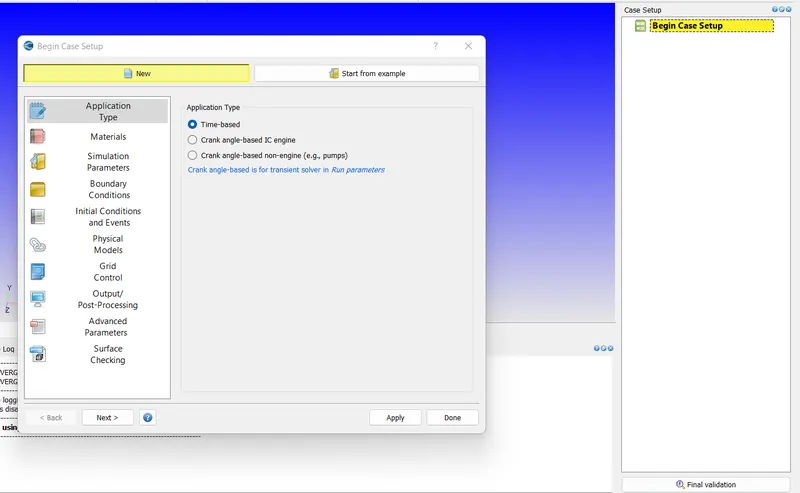
Now setting up the case study
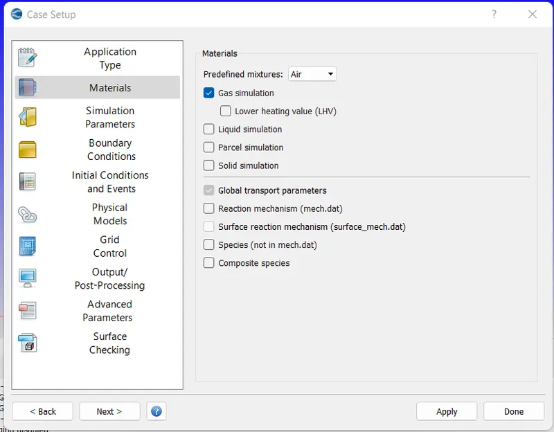
For materials there is no reaction mechanism and select Air
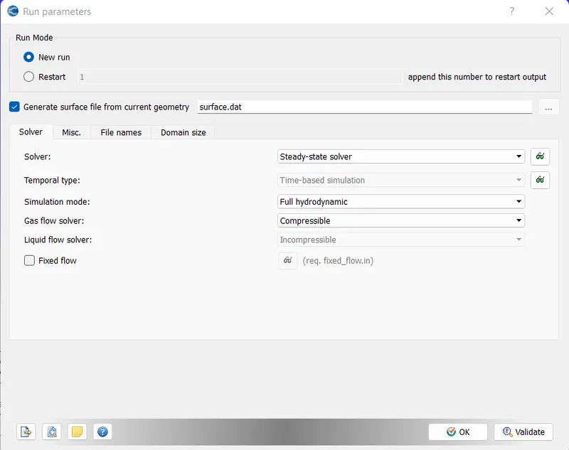
Simulation parameters are Steady state with full hydro dynamic compressible
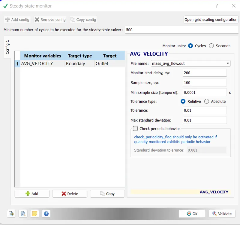
disabling solver species and enabling steady state monitor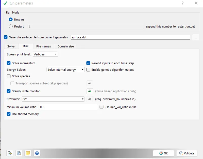
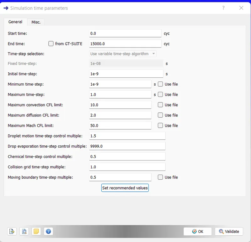
Giving simulation time parameters
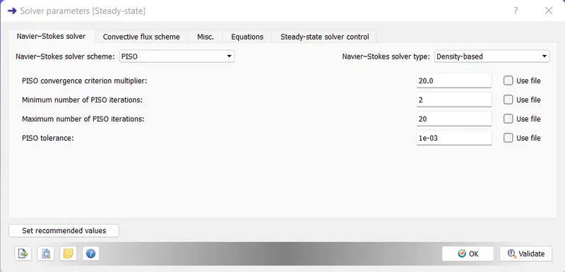
For solver parameters are at default
BOUNDARY DEFINATION:
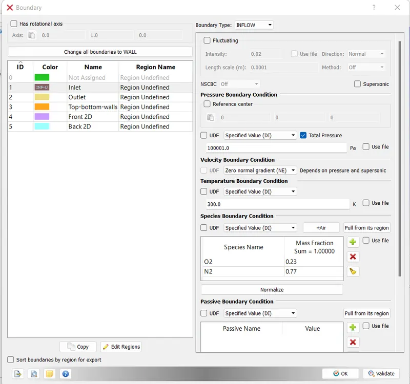
For Inlet, Boundary type is Inflow with 1Pa above 1bar i.e 100001 pa with Air
For outlet, Boundary type is out flow with 1bar pressure i.e 100000 Pa
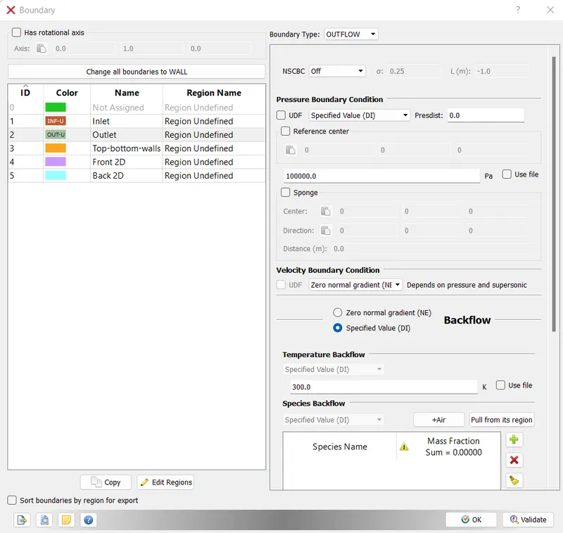
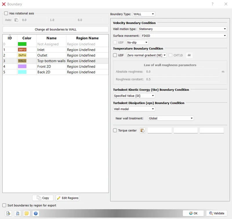
For top and bottom as boundary type wall
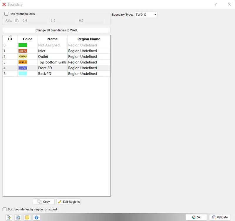
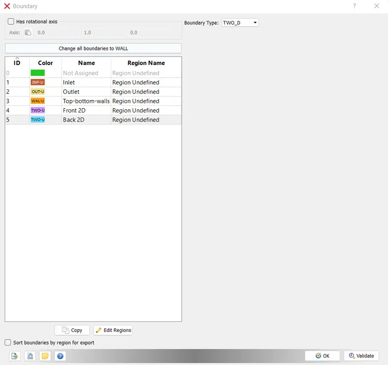
For front and back as two-D
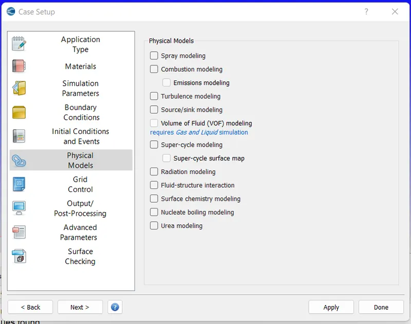
Unchecking the turbulence model in physical model
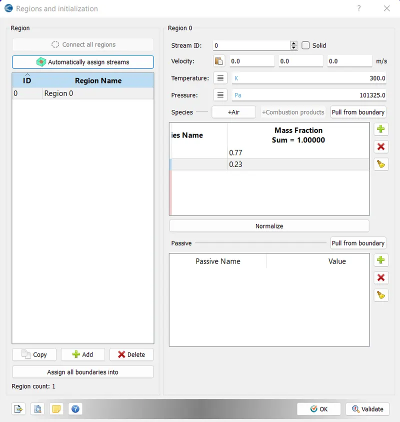
Regions and initialization we change the mass fraction of O2 and N2
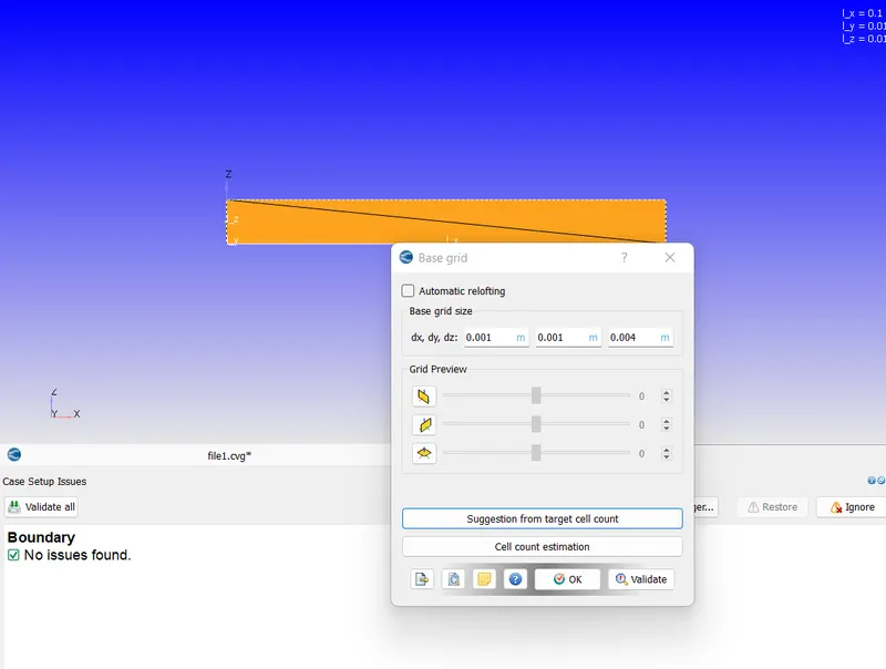
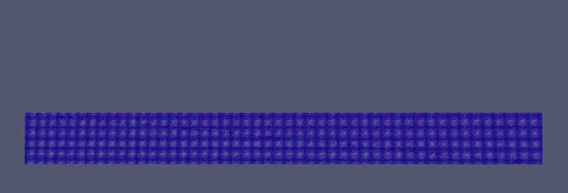
Giving base grid conditions in x-direction 100 cells i.e 0.1/100=0.001 and in y-direction 10cells 0.01/10=0.001 we are not concerned about in z-direction
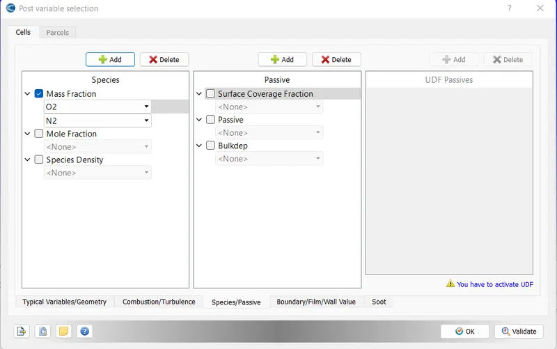
Post variable selections
With default and adding O2 and N2 species in the mass fractions
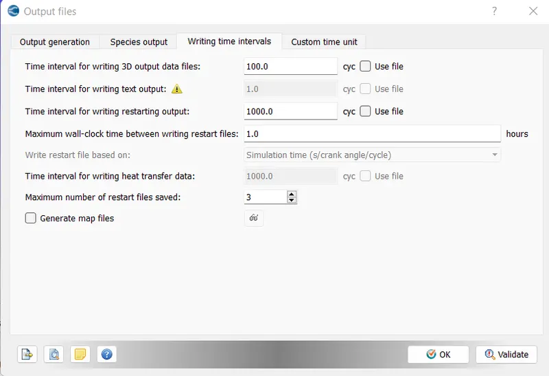
For output files
Time interval for writing 3D is 15000/100=150 ouput files
For steady state monitor
Solver parameters
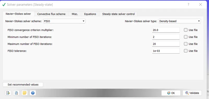
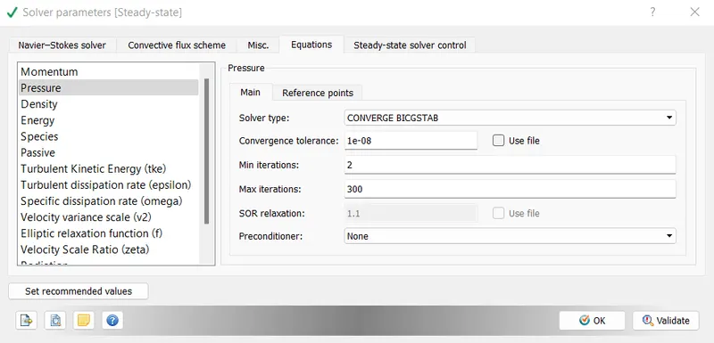
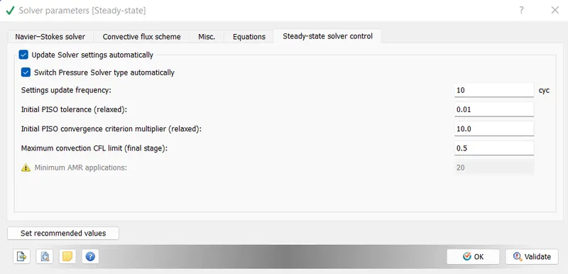
Then to run each case using solver 'mpiexxec.exe' and 'converge.exe' and post process results using 'mpiexec.exe' amd 'post_convert_30_serial_64.exe'.
CASE-1:
with mesh size of dx=dy=dz=2e-4
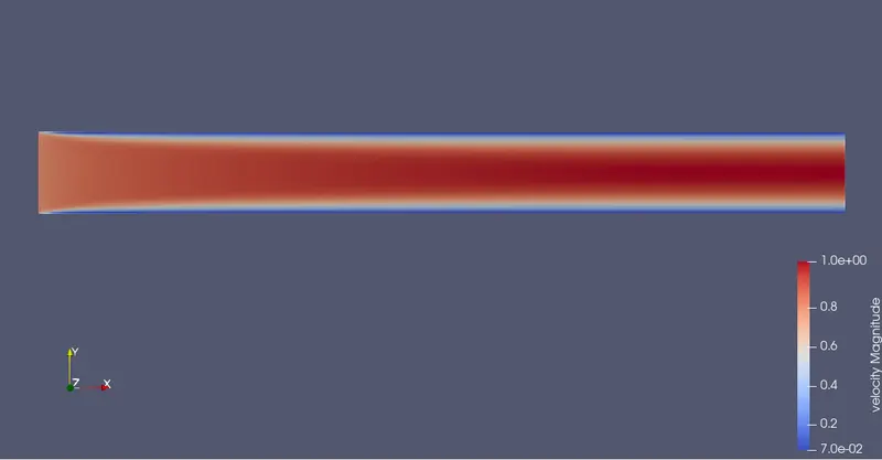
Velocity contour is
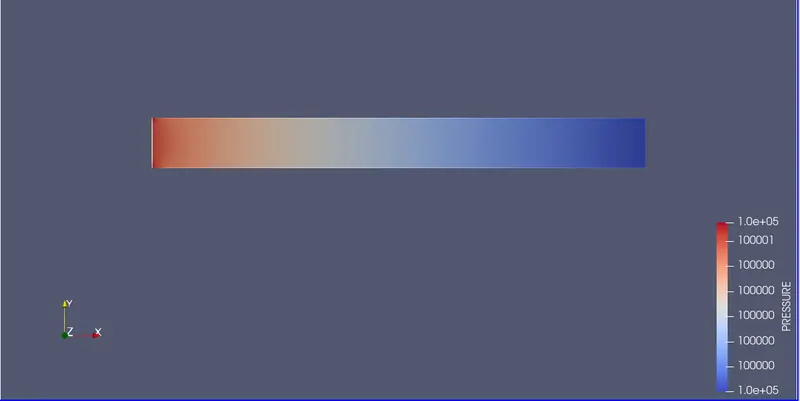
Pressure contour is
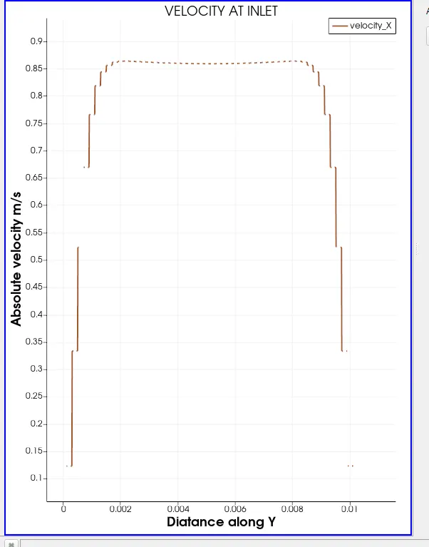
Velocity plot at inlet
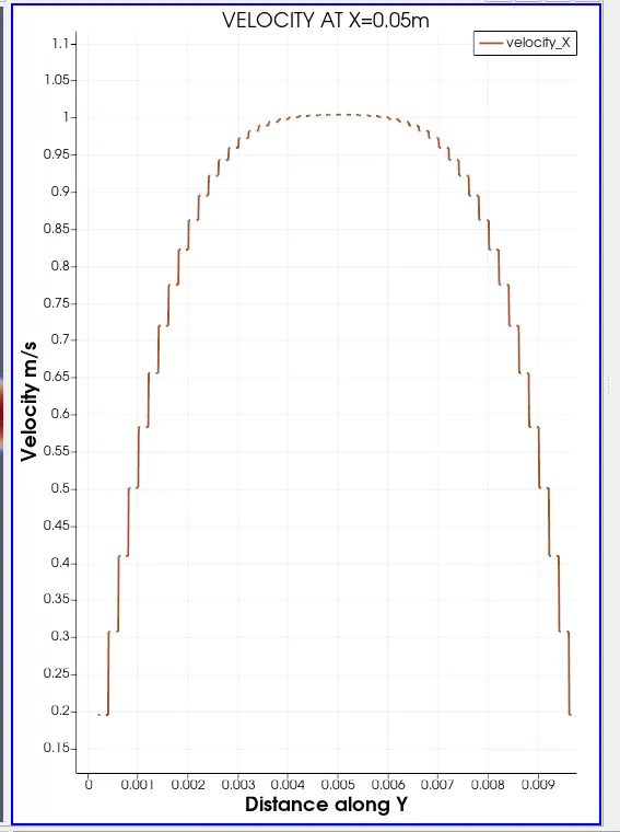
Velocity plot at 0.05m
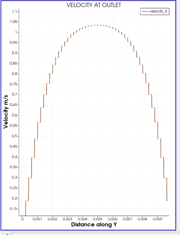
Velocity at outlet
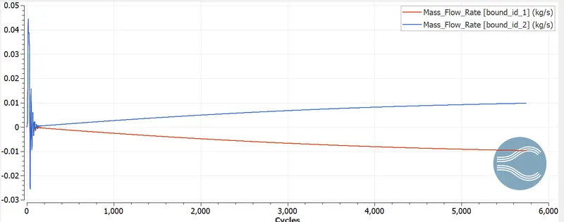
Mass flow rate at 1-inlet and 2-outlet
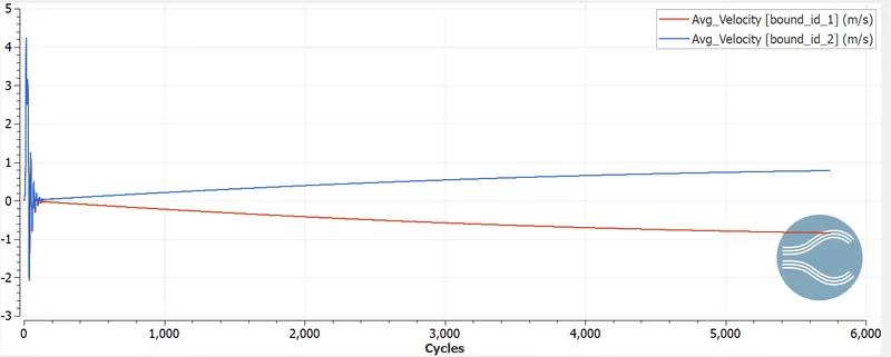
Average velocity at 1-inlet and 2-outlet
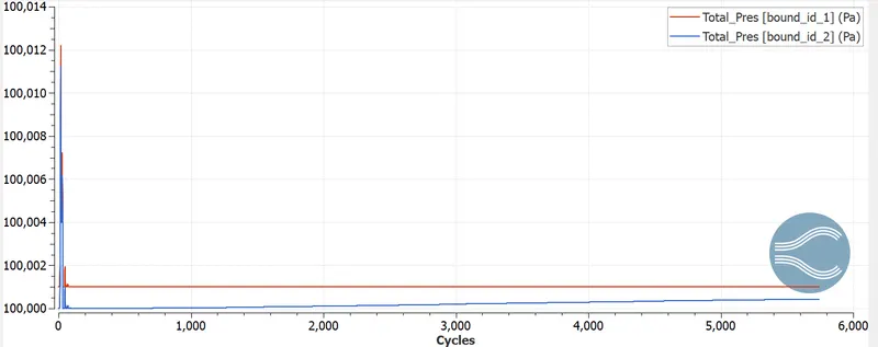
Total pressure 1-at inlet and 2-at outlet
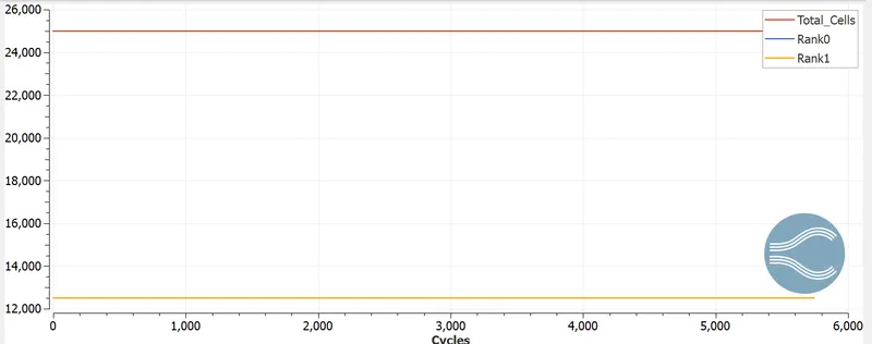
Cell count
CASE-2:
with mesh size of dx=dy=dz=1.5e-4
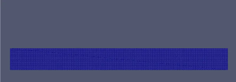
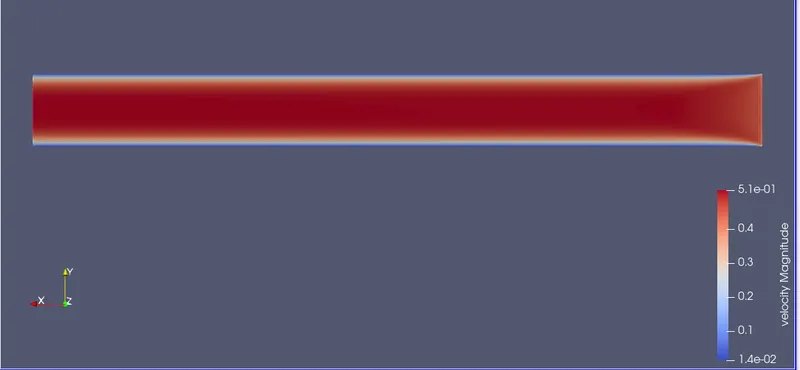
velocity contour is
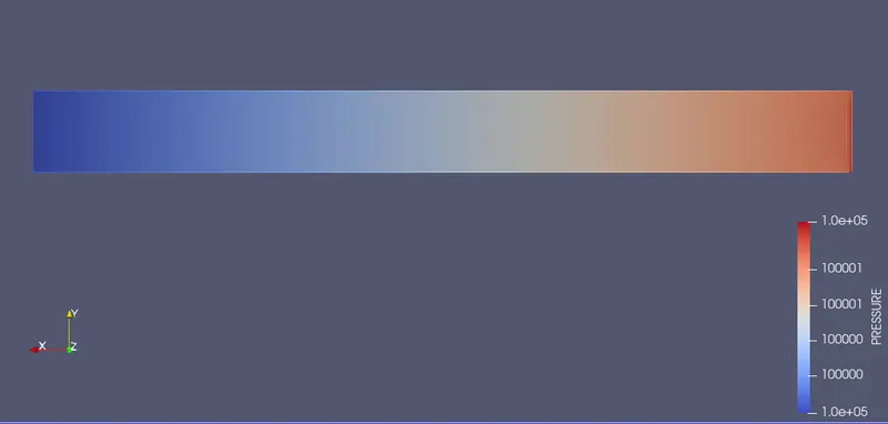
Pressure contour is
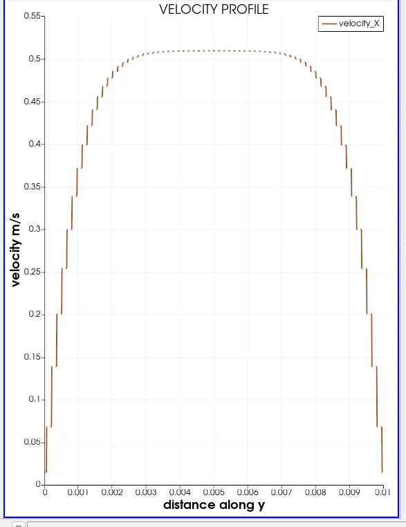
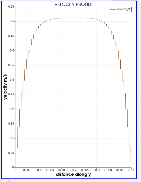
Velocity at inlet
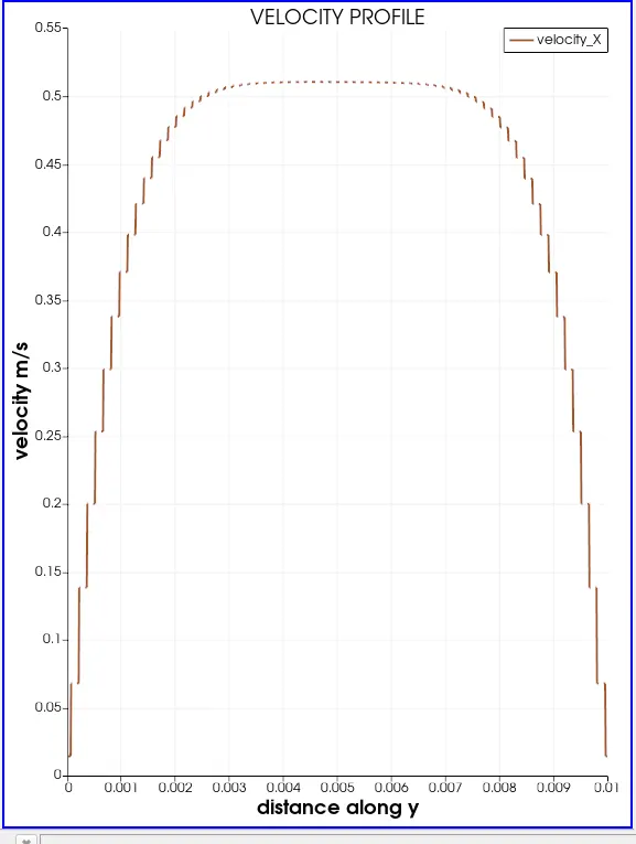
Velocity at 0.05m
Velocity at outlet
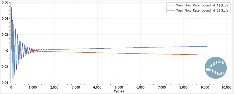
Mass flow rate 1-at inlet and 2-at outlet
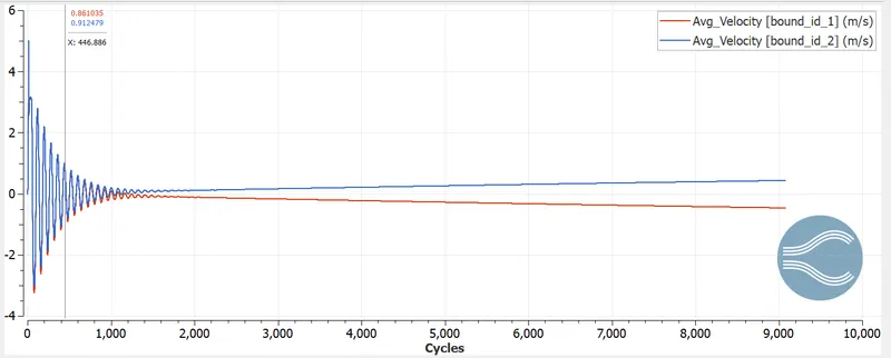
Average velocity 1-at inlet and 2-at outlet
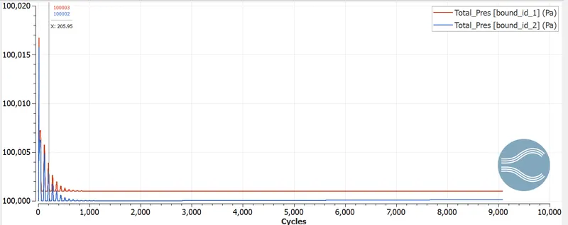
Total pressure 1-at inlet and 2-at outlet
Cell count
CASE-3:
with mesh size of dx=dy=dz=1.2e-4
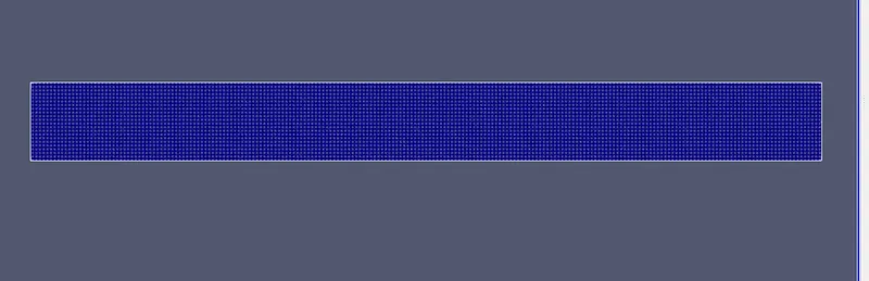
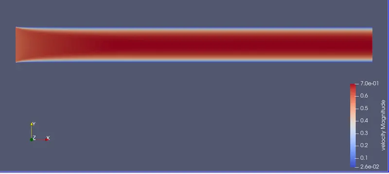
velocity contour is
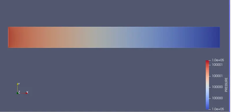
Pressure contour is
Velocity at inlet
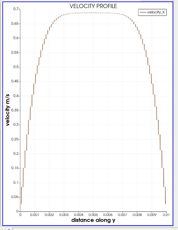
Velocity at 0.05m
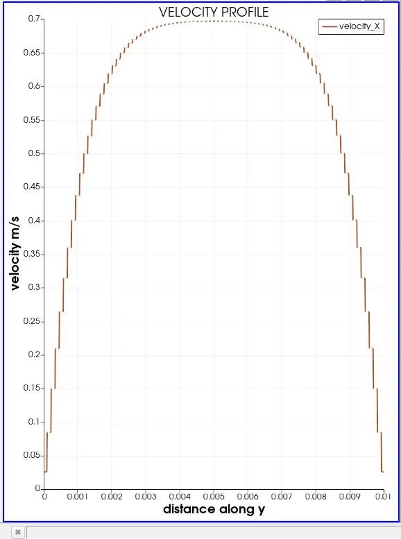
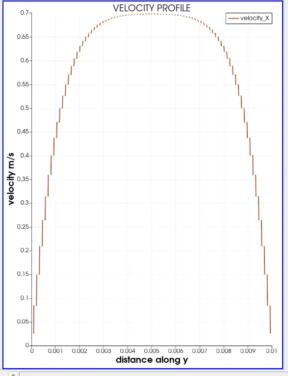
Velocity at outlet
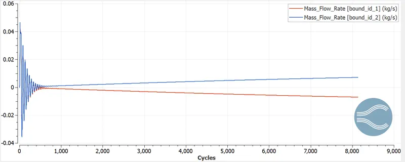
Mass flow rate 1-at inlet and 2-at outlet
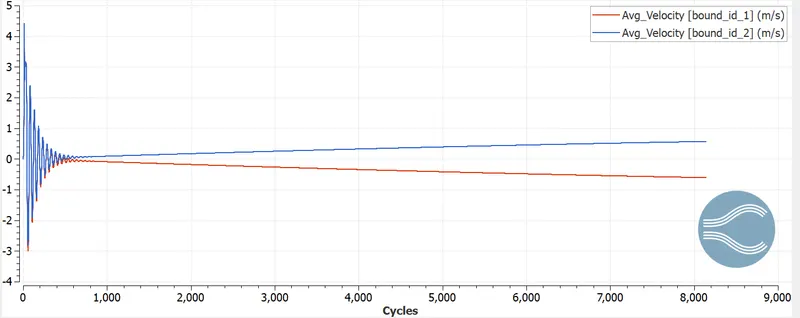
Average velocity 1-at inlet and 2-at outlet
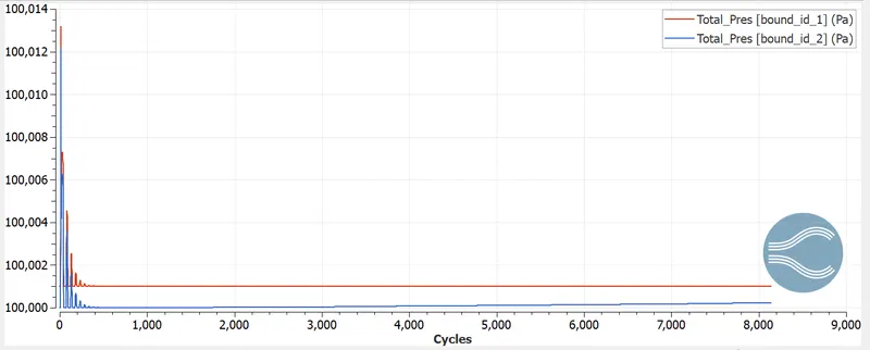
Total pressure 1-at inlet and 2-at outlet
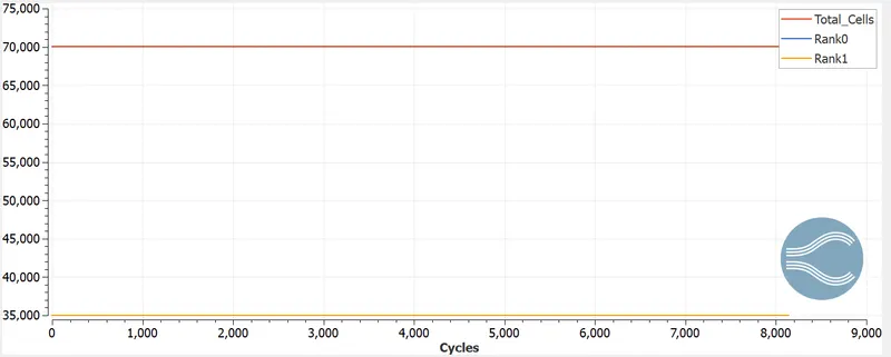
Cell count
OBSERVATIONS AND CONCLUSION:
Pressure difference between the inlet and outlet is what causes the flow in the channel.
From the contour plots of velocity the velocity at different instances, we observe that at the inlet the profile is flat and as we move across the channel for inlet to outlet, the profile develops into its characteristic parabolic curve and continues till outlet.
From the velocity contours we observe that the regions adjacent to the wall, the fluid velocity is zero.This is due to no slip condition of walls we defined.As we move across the channel the thickness of the fluid region which is at rest increases.
In the profile of mass flow rate and average velocity at the inlet and outlet are of similar profile.However the plots are inverse of each other in accordance with laws of conservation of mass.
From total pressure plot we see that pressure at inlet remains constant and pressure at outlet marginally increases during the cycle.
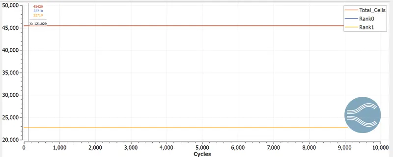
The cell count for the three cases remained constant during the simulation indicating that cells were intact during the computational simulation.
With the refinement of mesh we observe increase in computational time.
From the animations recorded we understant how the velocity profile develops. Initially it is zero everywhere in the fluid flow and with time we observe changes in the channel like no slip region and irrotational flow region.