Week 3 - Solving second order ODEs
AIM: To write a program in Matlab that will simulate the pendulum motion
DESCRIPTION:
In Engineering, ODE is used to describe the transient behavior of a system. A simple example is a pendulum
The way the pendulum moves depends on the Newtons second law. When this law is written down, we get a second order Ordinary Differential Equation that describes the position of the "ball" w.r.t time.
PROGRAM TO SIMULATE PENDULUM WITH ODE FUNCTION
% To Write a program in Matlab that will simulate the pendulum motion
clear all
close all
clc
% Simple pendulum inputs
b=0.05; % damping co-efficient
m=0.1; %mass of pendulum ball in kg
g=9.81; %gravity on ball in m/s^2
l=1; %length if the pendulum string in m
% Initial conditions angular displacement=0m angular velocity=3m/s
theta_0 = [0;3];
%time points from 0 to 20seconds
t_span = [0 20];
%solve ODE
%Ode is a inbuilt solver in matlab with main variables time(t),theta
%ode_func is used to make 2nd order to 2st order
[t, results] = ode45(@(t,theta) ode_func(t, theta, b, g, l, m), t_span, theta_0);
figure(1) %to get the velocity-acceleration time domain graph
hold on
plot(t,results(:,1));
plot(t, results(:,2));
xlabel('time');
ylabel('plot');
legend('Velocity', 'Acceleration'); % to define which graph shows what
video = VideoWriter('animation.avi','Uncompressed AVI'); %saved with file name and file resolution
video.FrameRate = 60; %a frame rate of 60frames per second is used
open(video)
% Origin
figure(2)
x0 = 0; % initial orgins of the pendulum
y0 = 0;
for i = 1:length(t) %from origin to the length of the pendulum
x1 = l*sin(results(i,1)); %along x-axis
y1 = -l*cos(results(i,1)); %along y-axis opposite direction
plot(x0,y0,'Marker','s'); % at origin with square mark
hold on %hold on use to take all previous lines in consideration
plot(x1,y1,'Marker','o'); %at end with circle mark for ball
plot([x0 x1],[y0 y1]); %to join origin and end
axis([-2 2 -2 2]) %axis is moves to get clear animation
pause(0.02);
hold off %hold off is used because to not leave the prints of pendulum for each frame
writeVideo(video,getframe(gcf)); %video is written on the disk
end
close(video);
PROGRAM FOR ODE FUNCTION:
function[dtheta_dt] = ode_func(t, theta, b, g, l, m);
theta1 = theta(1);
theta2 = theta(2);
dtheta1_dt = theta2;
dtheta2_dt = -(b/m)*theta2-(g/l)*sin(theta1);
dtheta_dt = [dtheta1_dt;dtheta2_dt];
end
ERRORS:
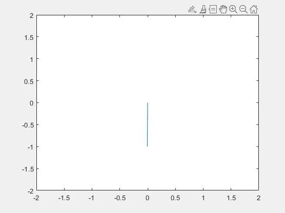
if hold on is not used after giving the end and origin of pendulum the prior program lines are missed and the orgin is now with marker
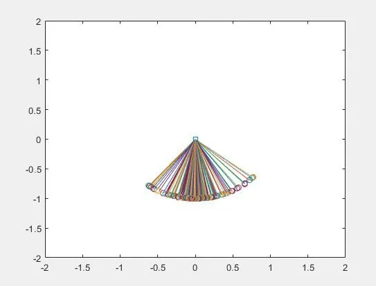
if hold off is not used before the end for loop, all the prints of the pendulum are traced in the animation. so to skip this hold offf is used
OUTPUTS:
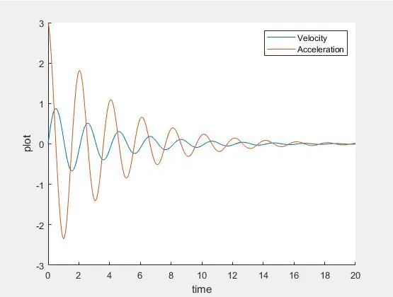
A velocity acceleration time domain graph with damped graph can be see. A legend command if used to show the differentiation in the graphs of each i.e velocity and acceleration