Simulating Channel Flow using Converge CFD
SIMULATING CHANNEL FLOW USING CONVERGE CFD.
INTRODUCTION
Channel flow is an internal flow in which the confining walls change the hydrodynamic structure of the flow from an arbitrary state at the channel inlet to a certain state at the outlet. The simplest illustration of internal flow is a laminar flow in a circular tube, while a turbulent flow in the rotor of a centrifugal compressor is an example of the most intricately shaped internal flow. Engineering devices employ channels with cross-sections of various geometrical shapes. In this project, Converge Studio was used to establish a working idea of airflow simulation through a channel flow under certain parameters, which will be elaborated systematically in this report.
OBJECTIVES
- Setup channel flow simulation.
- Run simulation for 3 different mesh sizes.
- Plot velocity and pressure contours for all 3 mesh sizes.
- Show plots for velocity, pressure, mass flow rate, and total cell count for all 3 mesh sizes.
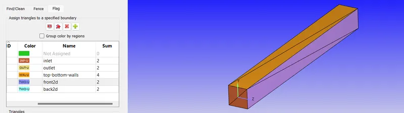
The laminar flow in a pipe is a very simple problem which can be a good problem to start with learning a new CFD software. In this report, a channel flow is simulated for 3 mesh sizes. The analysis is in 2D, so the shape of the cross-section of the channel won't matter. So, a cuboidal channel is created with a length of 0.1 m and a cross-section of 0.01 x 0.01 m. The box type geometry option is considered with triangular units. The image below shows the image of the computational domain with its named boundaries.
BOUNDARY FLAGGING:
The boundaries are flagged. The converge studio basically uses triangular blocks to create geometry. So by selecting the boundaries of the triangle are Flagged.
- Inlet
- Outlet
- Top and Bottom Walls
- Front2D
- Back2D
BOUNDARY:
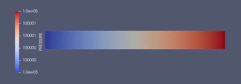
Inlet: Inflow boundary condition with pressure inlet at 100001 Pa.
Outflow: Outflow boundary condition with pressure outlet at 100000 Pa
Top and Bottom: No Slip walls.
Front and Back: 2D faces. (It tells solver to not solve in Z direction)
Initial region pressure = 100000 pa
CASE SETUP:
- Application Type = Time-based
- Materials- Air
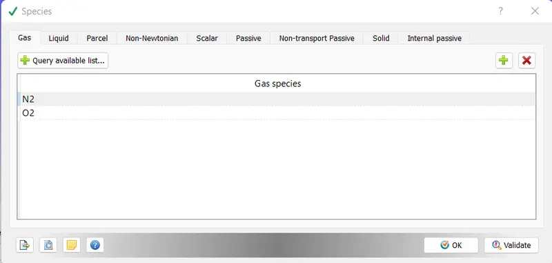
- Gas simulation is checked.
- The species O2 and N2 were entered from checklist.
- Simulation Parameters
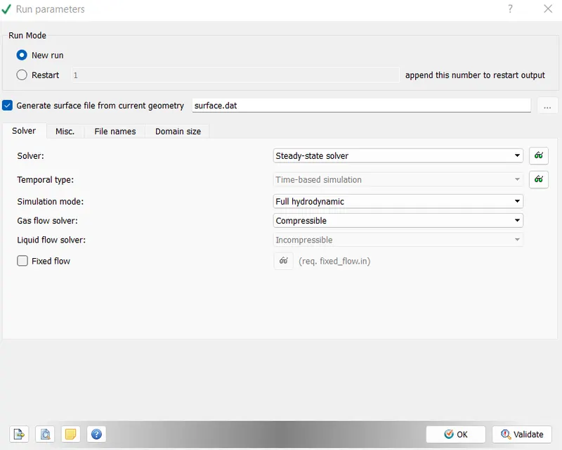
In Run Parameters- two main things to be considered
(a). Select the following solver settings.
- STEADY-STATE MONITOR
In order to run a steady-state/ transient simulation, firstly under the application type in the setup tree, a time-based simulation is selected.
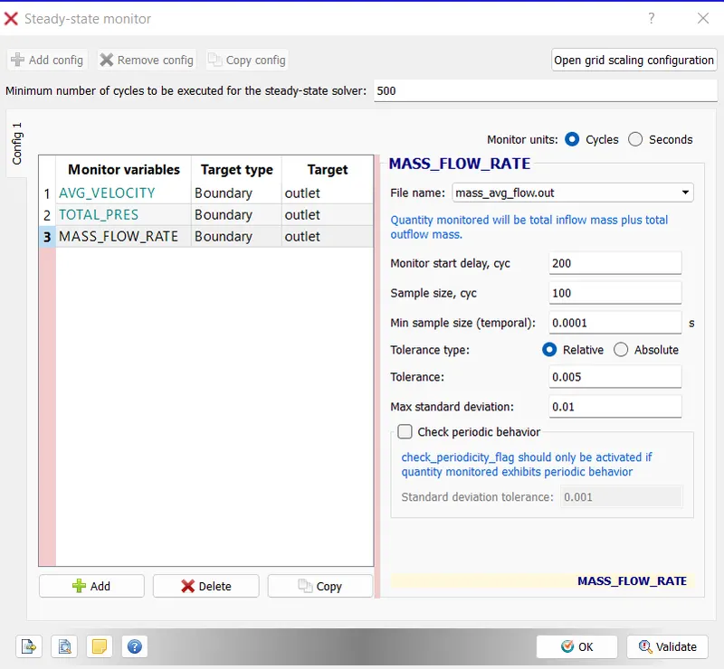
It is a mandatory option in Converge 3.0 for Steady-State simulations in order to assess the convergence of the simulation after it has converged.
The option to turn the steady-state monitor "On" is available under the miscellaneous tab.
Steady State monitor properties: (Used to stop the simulation when the difference between two monitor variable values in the sample is lower than tolerance)
Monitor variable: Average Velocity at outlet calculated from mass average flow output file.
Monitor start delay: 200 cycles
Sample size: 100 cycles
Relative Tolerance: 0.005
------------------------------------------------------------------------------------------------------------------------------
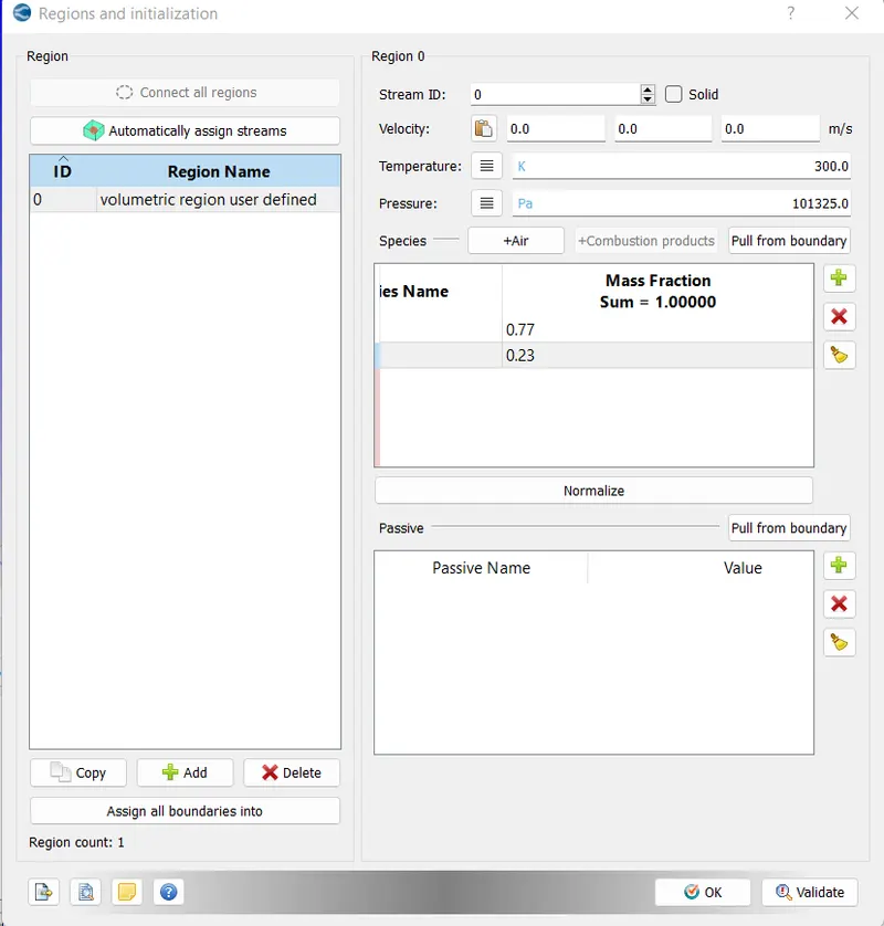
- REGIONS AND INITIALIZATION:
Temperature:300 K
Pressure:101325 Pa
Species mass fractions of O2 and N2 are interchanged to O2=0.77 and N2=0.23 to verify how steady-state changes the mass fractions of N2 and O2.
Physical Models: Uncheck Turbulence Modeling in this Case.
Grid Models: Grid is defined based on the different mesh sizes given in the project assignment.
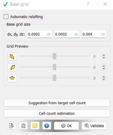

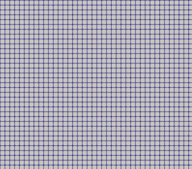
0.0002 X 0.0002 X 0.0002 0.00015 X 0.00015 X 0.00015
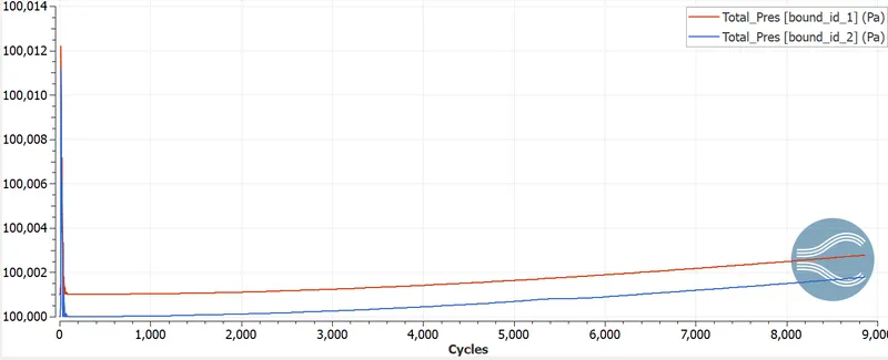
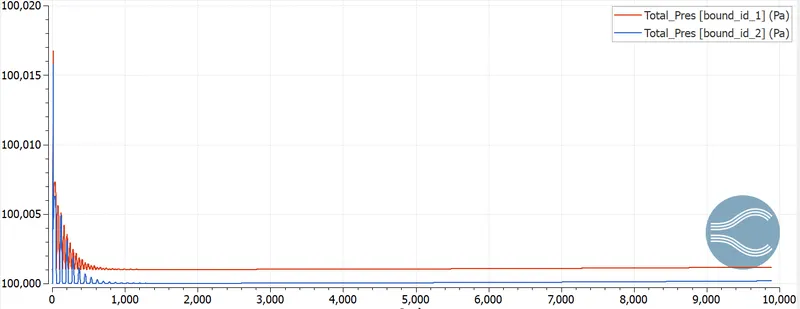
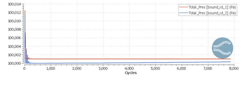
POST-PROCESSING for mesh size 0.0002,0.00015 and 0.0001 Respectively
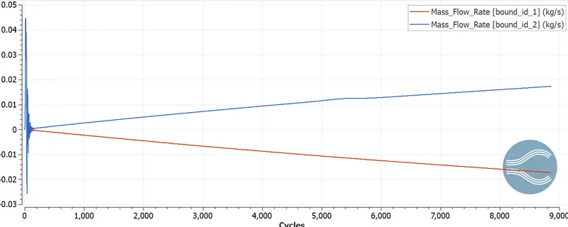
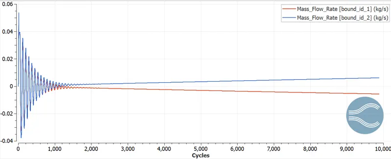
GRAPHS OF MASS FLOW RATE
----------------------------------------------------------------------------------------------------------------------------
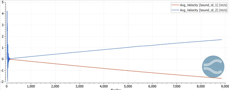
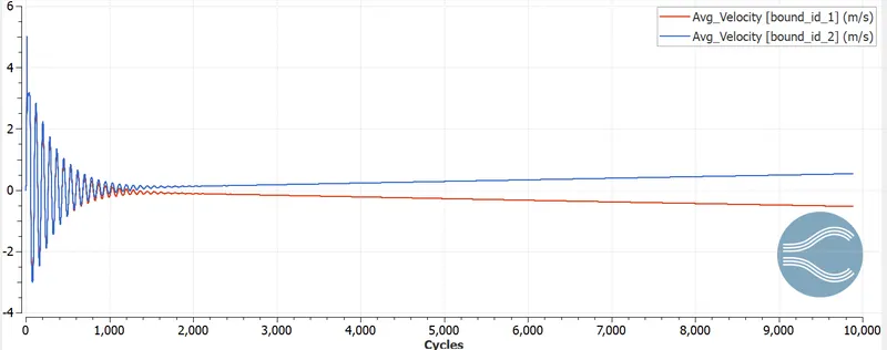
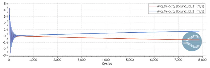
AVERAGE VELOCITY
------------------------------------------------------------------------------------------------------------------------------
TOTAL PRESSURE
------------------------------------------------------------------------------------------------------------------------------
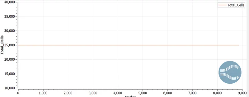
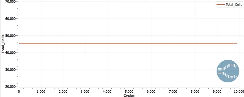
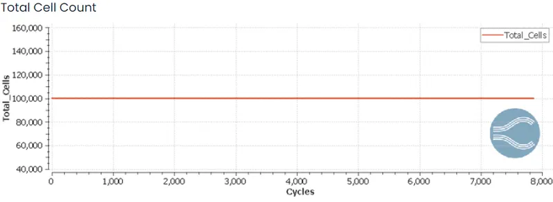
CELL COUNT
-----------------------------------------------------------------------------------------------------------------------------
Velocity

---------------------------------------------------------------------------------------------------------------------------
Pressure
-----------------------------------------------------------------------------------------------------------------------------
Velocity Flow Development Animation:
-----------------------------------------------------------------------------------------------------------------------------
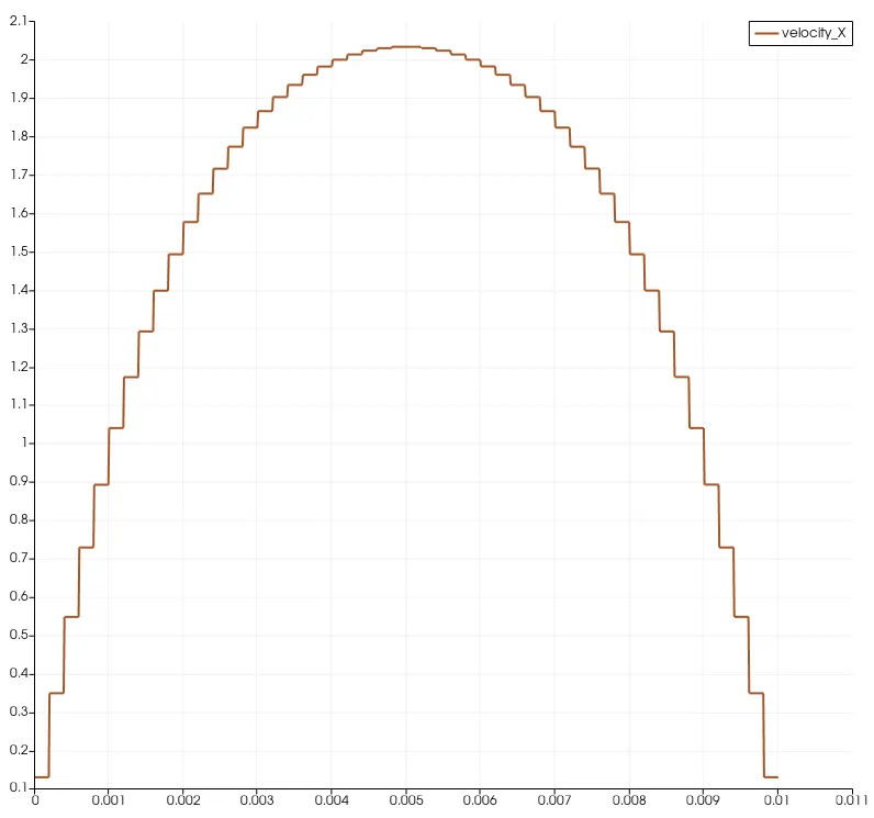
Velocity profile
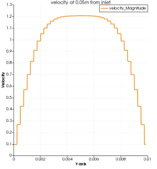
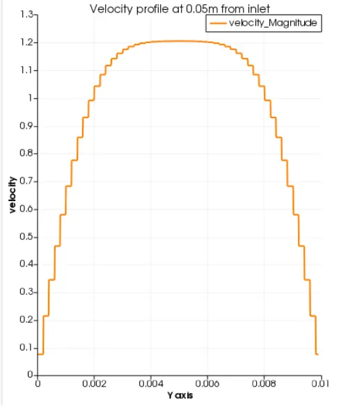
0.00015m 0.00012m
----------------------------------------------------------------------------------------------------------------------------
OBSERVATIONS:
- It is clear from the results that for mesh sizes (2e-4, 1.5e-4, 1.0e-4) the total cell count for each of the mesh is 25000, 45000, and 100000 respectively. Hence as the mesh becomes finer and finer the total cell count increases, as the cell count increases the computational time also increases.
- It is observed that velocity in the initial case is highest but as the mesh is coarse it is generally not preferred to be accurate. Finer mesh results in more accuracy.
- The continuity equation was satisfied in all the cases.
- As the mesh becomes finer, the velocity profile obtained is also much clear compared to the other 2 cases.
- Hence, as the size increases the results obtained are much clear and more accurate.
CONCLUSION:
Results show accuracy with decreasing mesh size. It could be concluded that velocity, pressure, and mass fractions of oxygen and nitrogen become stable after convergence. The reversed mass fractions of O2 and N2 as initial conditions come to the universal state at the end of the simulation.