To calculate the hill climbing power ratio for TATA ultra truck an d Model A WOT for GM EV1

Aim:

1. To Calculate the ratio of power for hill-climbing for a fully loaded TATA Ultra truck to a half-loaded truck.
2. To calculate the minimum length of the flyover.
3. To prepare a drive cycle using an excel sheet and get the output using the drive cycle model.
4. To model a Wide-open throttle (WOT) for a GM EV1 car.

RATIO OF HILL CLIMBING POWER FOR A TATA ULTRA TRUCK FOR FULLY LOADED AND HALF LOADED TRUCK

INTRODUCTION

T.10 Ultra is launched at 9600 GVW is the best fit as a short, city, and medium-haul transportation for shorter wheelbases like 33, 39, medium, and long haul for 45 and 49 WB. It is developed to delight both the fleet owners as also the general driving fraternity. 5-speed G550 gearbox optimized ratios and optimized operating temp for FE improvement.

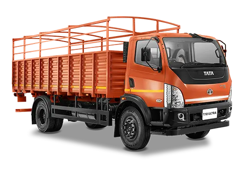
Technical Specification

For the calculation of the hill power, we required the two most important parameters i.e weight of the truck and the gradability.

Governing Equations

• Hill climbing force

`F_hc = m * g *sin φ`

• Power required for hill climbing

`p_hc = F_hc * V`

• Gradability

`G= (Rise)/(Run) *100%`

Solution:

Given:

Gross weight (kg) = 9600

Kerb weight (kg) = 3250

Payload (kg) = 6350

Gradability = 30%

To find:

Hill climbing power ratio for full loaded to half loaded truck

Solution:

Assuming that the speed of the truck is constant at 30 kmph

= 30 * 5/18

= 8.333 mps

We know that

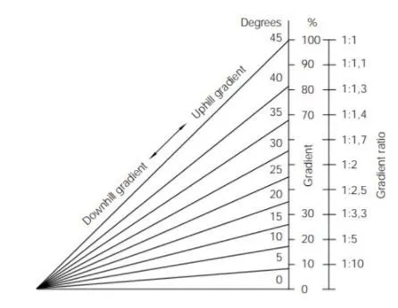
Gradebility = 30%

= 0.3

`G= (Rise)/(Run) *100%`

= `tan(θ)`

Here we can consider 0.3 as the inclination of angle

G = `tan^-1 (0.3)`

= `16.69^@`

For verifying the results

For full loaded condition

Gross weight (kg) = 9600

The hill-climbing force is

`F_hc = m * g *sin φ`

= 9600 * 9.81 * sin (16.69)

= 27046.72 N

Power required for hill climbing

`p_hc (FL) = F_hc * V`

= 27046.72 * 8.33

= 225299.18 W

= 225.29 KW

For half loaded condition

Payload = 6350 Kg

= 6350/2

= 3175 kg

GVW = 3175 + 3250

= 6425 Kg

The hill-climbing force is

`F_hc = m * g *sin φ`

= 6425 * 9.81 * sin (16.69)

= 18743.31 N

Power required for hill climbing

`p_hc (HL)= F_hc * V`

= 18743.31 * 8.33

= 156131.81W

= 156.1318 KW

Power ratio = `(p_hc (FL))/(p_hc (HL))`

= `(225.29)/156.1318`

= 1.4429

TO CALCULATE THE LENGTH OF THE FLYOVER

Given

minimum height of flyover (rise ) = 5.5 m

To find

Length of flyover

Solution

Assuming

Gradeability = `16.69^@`

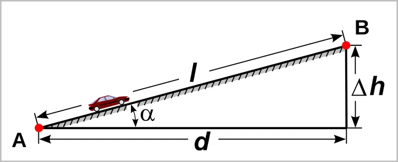
We know that

`tan ψ = (opp)/(adj)`

`tan(16.69)=(5.5)/(Run)`

Run = 18.34 m

`sin( ψ) = (opp)/(hyp)`

`Sin(16.69) = (5.5)/(Hyp)`

Hyp = 19.150 m

verification

`G= (Rise)/(Run) *100%`

= `(5.5)/(18.34) **100`

= 30%

Hence our calculation are verified

Using pythagorous

`L^2 = Rise ^2 + Run^2`

= `(19.15)^2 +(18.34)^2`

= 26.51 m

PREPARE A DRIVE CYCLE AND PLOT THE VELOCITY AND TIME USING SIMULINK

Procedure

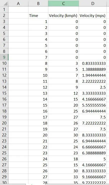
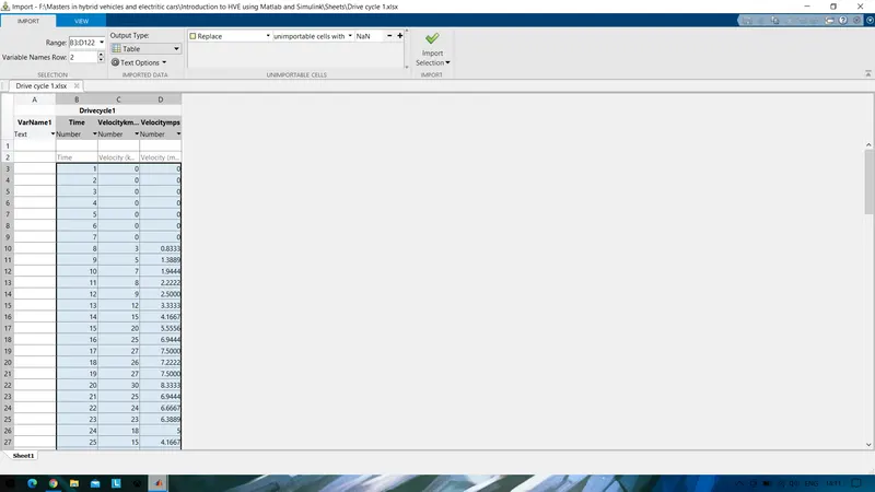
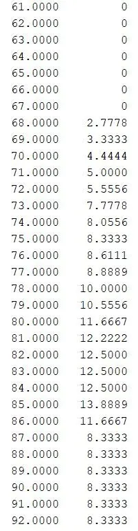
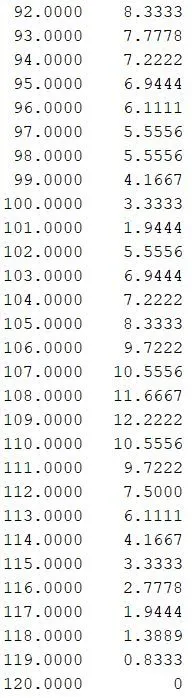
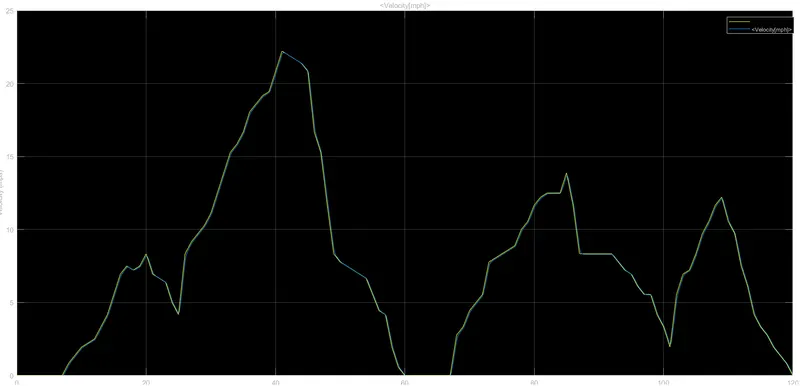
• Prepare a drive cycle for 120 seconds and velocity corresponding to that time frame using excel.
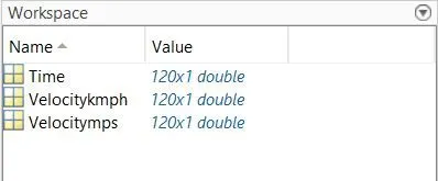
• Import the data in the excel sheet to Matlab for different vectors of velocity and time to the workspace.
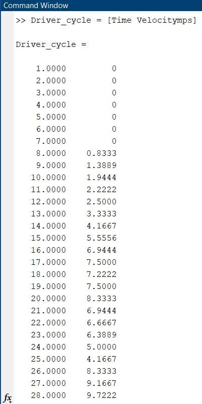
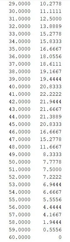
• Now convert the imported data to an array in Matlab.

• Excel Sheet

• Imported data to Matlab

OUTPUT

Workspace

Command window

Driver Glider

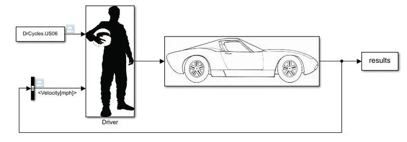
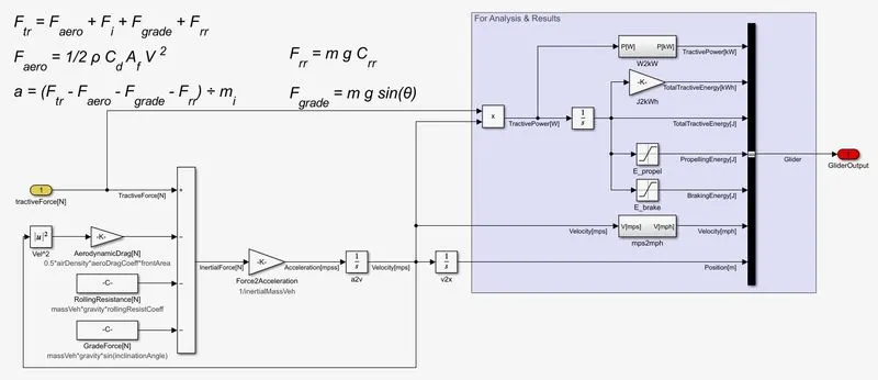
• Download the vehicle modeling file and extract the data and add it to the MATLAB
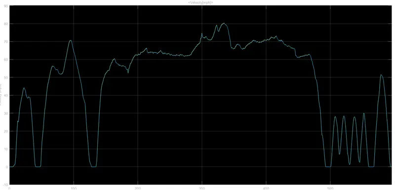
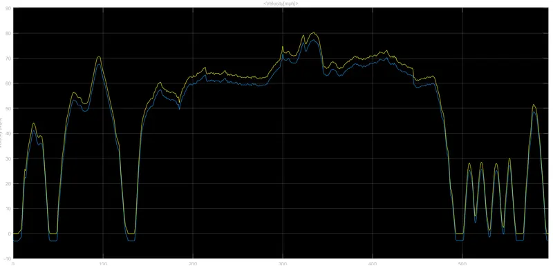
• Open the Driver_glider.slx and change the angle to 14 degrees and run the simulation
• Observe the plot before and after changing the angle.
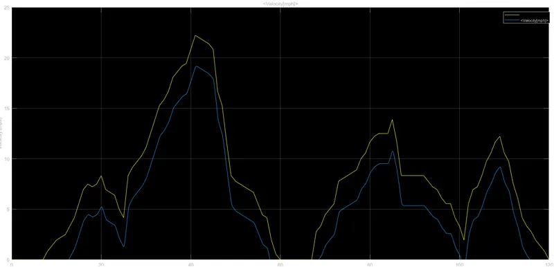
• Next include the driving cycle that we created and repeat the process for the new drive cycle.

Original Driver- glider

Glider

OUTPUT:

Before changing the angle (original driver cycle)

After changing angle to 14 degree

Including the new drive cycle

MODEL WIDE OPEN THROTTLE FOR GM EV1 CAR

Vehicle parameters

• Drag coefficient Cd = 0.19
• rolling resistance R = 0.048
• Vehicle mass (m) = 1540 kg
• Gera ratio G = 11
• Radius of tire r = 0.30
• motor torque Tmax = 140 Nm
• Max speed = 1200 rmp
• Critical velocity Vc = 19.8 m/s
• Frontal area A = 1.8 m^2
• Efficiency E = 0.95

Parameters after 5% change

• Drag coefficient Cd = 0.1995
• rolling resistance R = 0.00024
• Vehicle mass (m) = 1617 kg
• Gera ratio G = 11.55
• Radius of tire r = 0.315
• motor torque Tmax = 147 Nm
• Max speed = 12600 rmp
• Critical velocity Vc = 20.79 m/s
• Frontal area A = 1.89 m^2

Governing equations

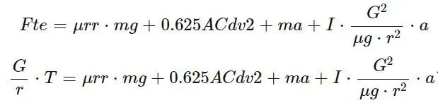
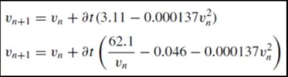
Code:

%Wide open throttle (WOT) response
clear  all
close all
clc
%Input 
%Drag coefficient 
Cd = 0.19;
%Rolling Resistance 
r = 0.0048;
%Vehicle Mass 
m = 1540;
%gear ratio 
g = 11;
%Radius of tire (r)
rt = 0.30;
%motor Torque 
Tmax = 140;
%critical Velocity 
Vc = 19.8;
%frontal area 
a = 1.8;
%efficiency of the single speed drive 
E = 0.95;
%time 
t = linspace(0,120,300);
%Initial velocity 
v1 = 0;
dt = 0.1;
for n =1:299
    if v1(n)<19.8
        v1(n+1)=v1(n)+dt*(3.11-(0.00137*(v1(n)^2)));
    else
        if v1(n)>=19.8
            v1(n+1)=v1(n)+((62.1/(v1(n))-0.046-(0.000137*(v1(n)^2))));
        end
    end
end
%plotting
figure(1)
plot (t,v1);
title ('WOT of Gm Ev1')
xlabel ('time (sec)')
ylabel ('Velocity (m/s)')
grid on 

%WOT with 5% changes 
%Input 
%Drag coefficient 
CD = 0.1995;
%Rolling Resistance 
R = 0.00024;
%Vehicle Mass 
M = 1617;
%gear ratio 
G = 11.55;
%Radius of tire (r)
RT = 0.315;
%motor Torque 
TMAX = 147;
%critical Velocity 
VC = 20.97;
%frontal area 
A = 1.89;
%velocity
v2 = (v1*0.05)+v1;

if v2(n)<20.97
    v2(n)=v2(n)+dt*(2.95-(0.000137*(v2(n)^2)));
else if v2*(n)>=20.97
        v2(n+1)=v2(n)+dt*((59.14)/v2(n)-0.046-(0.0001137*(v2(n)^2)));
    end
end
%plotting
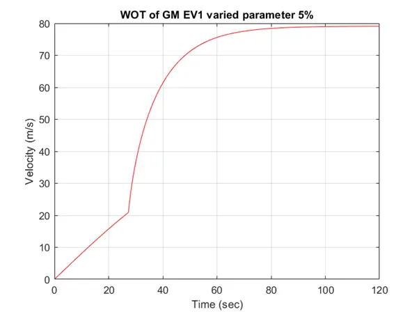
figure(2)
plot(t,v2,'color','r')
title('WOT of GM EV1 varied parameter 5%')
xlabel('Time (sec)')
ylabel('Velocity (m/s)')
grid on

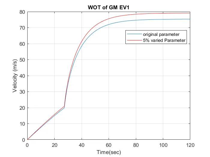
figure(3)
plot (t,v1);
hold on
plot(t,v2,'color','r')
title('WOT of GM EV1')
legend ('original parameter','5% varied Parameter')
xlabel('Time(sec)')
ylabel ('Velocity (m/s)')
grid on 

Explanation:

• Initially, the vehicle parameters are provided as the given data.
• Later velocity is calculated for the time frame of 120 seconds by providing the conditions as velocity.
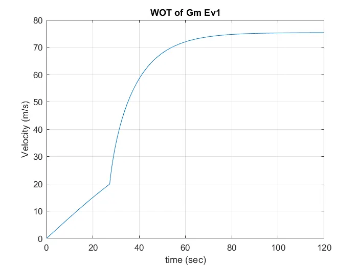
• Plot the velocity vs time graph for the acquired results.
• Later change the parameters by 5% of the original value.
• Plot the graph for the change parameters and compare it with the previous graph.

OUTPUT

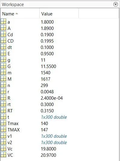
Workspace

Original Parameters

Changed parameters 5%

Combine graph

CONCLUSION:

From this exercise, we have calculated the hill-climbing power ratio for the tata ultra truck. Calculated the length of the flyover using the specifications of the truck. Created our own driver cycle and got the output using the Simulink block and observe the changes in the parameters. Successfully modeled the WOT for GM EV1 car and plotted the velocity VS time graph by varying the parameters of the car.