Plotting OTTO cycle and calculating the efficiency of the petrol engine.

AIM - To plot the OTTO cycle for a petrol engine and calculating the efficiency.

INTRODUCTION -

The Otto cycle is the ideal cycle for a spark-ignition reciprocating engine. It is named after Nikolaus A. Otto who builds a successful four-stroke engine in 1876 in Germany using the cycle proposed by Frenchman Beau de Rochas in 1862. In the most spark-ignition engine, the piston executes four complete strokes within the cylinder, and the crankshaft completes two revolutions for each thermodynamics cycle. these engines are called four-stroke internal combustion engines. The schematic of each stroke as well as the P-V diagram for an actual four-stroke spark-ignition engine is given below.

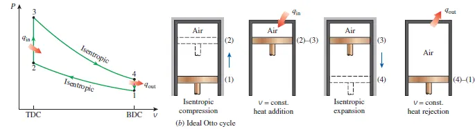
Initially, both the intake and the exhaust valves are closed and the piston is at its lowest position (BDC). During the compression stroke, the piston moves upward, compressing the air-fuel mixture. shortly before the piston reaches its highest position (TDC), the spark plug fires and the mixture ignites, increasing the pressure and temperature of the system. The high-pressure gases force the piston down, which in turn forces the crankshaft to rotate, producing a useful work output during the expansion or power stroke. At the end of this stroke, the piston is at its lowest position, and the cylinder is filled with combustion products. Now the piston moves upward one more time purging the exhaust gases through the exhaust valve, and down a second time, drawing in the fresh air-fuel mixture through the intake valve. Notice that the pressure in the cylinder is slightly above the atmospheric value during the exhaust stroke and slightly below during the intake stroke.

GOVERNING EQUATIONS-

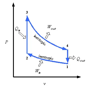
1-2 ISENTROPIC COMPRESSION

The piston moves from BDC to TDC, compressing the air-fuel mixture. The equations used for the calculation during this calculation are

`P*V ^ γ =` Constant (1)

`(P_1 V_1) / T_1 = (P_2 V_2) /T_2` (2)

The mixture is compressed inside the cylinder which changes the volume and increases the pressure in the chamber.

2-3 CONSTANT VOLUME HEAT ADDITION

Here the compressed mixture is supplied heat with come external source, this suddenly increases the temperature and pressure inside the chamber. This is a constant volume process

hence `V_2 = V_3`

the pressure is calculated using the ideal gas equation

`(P_3 V_3) / T_3 = (P_2 V_2) /T_2`

3-4 ISENTROPIC EXPANSION

As the temperature and the pressure inside the chamber increase the piston is pushed down for the TDC to BDC, this is known as the expansion stroke or the working stroke. This downward motion of the piston moves the crankshaft and work is done.

the pressure is calculated using the equation

`P*V ^ γ =` Constant

4-1 CONSTANT VOLUME HEAT REJECTION

This is the exhaust stroke releasing the heat generated during the previous stroke, this is a constant volume process with the exhaust gases releasing out. This is the final cycle in the 4 stroke cylinder engine. After this process, the next cycle starts from the beginning.

hence `V_4 = V_1`

OTHER EQUATIONS USED -

• There is another equation for the change in the volume for changing the crank angle,

`V/V_c = 1 + 1/2 (r_c -1)[R + 1 - cosθ - (R^2 - sin^2θ)^0.5]`

• The thermal efficiency of the Otto cycle is calculated by the equation

η = `1- ((Q _r)/(Q_s))`

where Qr = heat rejected

Qs = heat supplied

CODE IN MATLAB -

First code for plotting the points -

For the code to execute first we need to plot the 4 stages of the process, or to say the 4 points in the Otto cycle graph.

clear all
close all
clc
%input variable
gamma = 1.4;
t3 = 2300;

%state variable point 1 
p1 = 101325;
t1 = 500;

%engine geometric parameter 
bore = 0.1;
stroke = 0.1;
con_rod = 0.15;
cr = 12;

% calcualting swept volume and clearence volume. 
v_swept = (pi/4)*bore^2*stroke;
v_clearance = v_swept/(cr-1);

v1 = v_swept + v_clearance; 
v2 = v_clearance; 

% state variable at state point 2 
%p2v2^gamma = p1v1^gmma
p2  = p1*cr^gamma;
%p1v1/t1 = p2v2/t2 t1 = p2*v2*t1/(p1*v1)
 t2 = p2*v2*t1/(p1*v1);
 
 %state variable at atate point 3 
 v3 = v2;
 %p3v3/t3=p2v3/t2, p3 = p2*t3/t2
 p3 = p2*t3/t2;
 
 %state variable at stage 4
 v4 = v1;
 %p3v3^gamma = p4v2^gamma, p4 = p3*(v3/v4)^gamma
  p4 = p3*(v3/v4)^gamma;
  figure (1)
  hold on 
  plot (v1,p1,'*','color','r');
  plot (v2,p2,'*','color','r');
  plot (v3,p3,'*','color','r');
  plot (v4,p4,'*','color','r');

EXPLANATION

• This code will help us to plot the 4 points of the otto cycle which will represent the 4 stages of the Otto cycle.
• The input parameters are T3 and gamma which will help us with the calculation.
• We will be assuming some engine parameters like bore, stroke, connecting rod length, compression ratio.
• Once we have decided the parameters we will first calculate the swept volume and the clearance volume of the cylinder. The swept volume is the volume of the cylinder while for clearance volume we have a standard relation.
• Now we can calculate the volume at stage 1.i.e. V1 just by adding the swept volume and clearance volume. V2 will be equal to the clearance volume of the cylinder that is the volume remaining after the piston reaches the TDC.
• At state point 2 we will be calculating the pressure and temperature at point 2 i.e. P2 and T2. For calculating these values we will be using the isentropic equation and the ideal gas law. At this moment we will be having P1, V1, T1, P2, V2, T2.
• After this, we will be moving to stage point 3. This process is a constant volume heat addition process so V2 =V3. P3 will be calculated using the ideal gas equation.
• From 3 to 4 will be the isentropic expansion. This will be the stroke that will be generating the power that is required. The increase in the temperature and pressure in their last stage will be resulting in the expansion stroke.
• At state 4 will be the constant volume heat rejection, here V1 = V4, and the p4 can be calculated using the PV^gamma = constant relationship. Once calculating this we will be having all the variables that are required.
• The next step will be plotting these variables on the chart. By using simple plot command we can easily plot the points.

OUTPUT

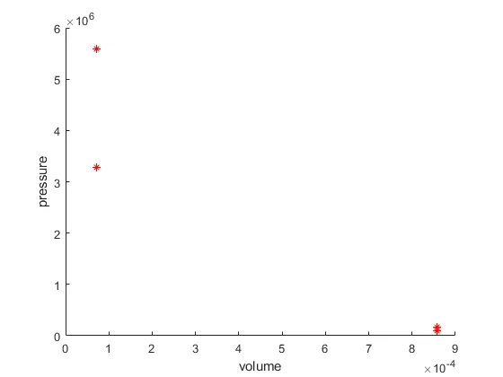
• The next step in this process will be joining these lines, but for that, we need to do some prior calculations of engine parameters and piston kinematics. We will be writing a function and later will be including the function in the final code which will get us the final result.

Function code -

%calculating the piston kinematics change in the volume inside the
%compression chamber. 

function [v] = engine_kinemetics(bore,stroke,con_rod,c_r,start_crank,end_crank)
a = stroke/2;
R = con_rod/a;
%calculating swept volume and clearance volume 
v_s = pi/4*bore^2*stroke;
v_c = v_s / (c_r-1);

theta = linspace(start_crank,end_crank,100); %angle of the crank at different position throught out cycle 
term1 = 0.5*(c_r -1);
term2 = R +1-cosd(theta);
term3 = (R^2-sind(theta).^2).^0.5; 

v = (1+term1*(term2-term3)).*v_c;  % change in the volume inside the chamber 
end

• This function is like a template that will be using the geometric parameters to solve the piston kinematics.
• For solving the piston kinematics we will be considering the complete crank angles from start to end. Hence we will use linespace command for generating the array.
• The change in the volume of the chamber is calculated from the equation mentioned above, that equation is completely generated from the geometric parameters.
• If this function is executed we will be having a complete array containing the change in volume inside the cylinder.

OUTPUT

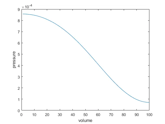
• This figure shows the change in the volume during the compression stroke of the piston. The volume doesn't vary linearly in the cylinder but in a curved profile.

Final code -

In the final code, we will be combining the two code mentioned above which will generate us the final results. we will be using the function that we generated in the first code and will solve for the output

clear all 
close all
clc
%Input variables 
t3 = 2300;
gamma = 1.4;

%stage 1 variables 
p1 = 101325;
t1 = 500;

%engine geometric parameters 
bore = 0.1;
stroke = 0.1;
con_rod = 0.15;
c_r = 12;

%calculating swept volume and clearance volume 
v_s = (pi/4)*bore^2*stroke;  
v_c = v_s / (c_r-1);
v1 = v_s +v_c;
v2 = v_c; 

%state variable at state point 2 (isentropic compression)
%p1v1^gamma=p2v2^gamma  
p2 = p1*c_r^gamma;
%p1v1/t1 = p2v2/t2
t2 = p2*v2*t1/(p1*v1);

%calculating compression volume and compression pressure 
constant_c = p1*v1^gamma;
V_compression= engine_kinemetics(bore,stroke,con_rod,c_r,180,0);
P_compression = constant_c./V_compression.^gamma;  %pv^gamma is constant along the isentropic process 

%state variable at stage 3 
v3 = v2;                                           %constant volume heat addition
%p3v3/t3 = p2v2/t2
p3 = p2*t3/t2;

%state variable at stage 4 (isentropic expension)
v4 = v1;                                            %constant volume heat rejection
%p3v3^gamma = p4v4^gamma 
p4 = p3*(v3/v4)^gamma;

%calculating expansion volume and expansion pressure 
constant_c = p3*v3^gamma;
V_expansion = engine_kinemetics(bore,stroke,con_rod,c_r,180,0);
P_expansion = constant_c./V_expansion.^gamma;  %pv^gamma is constant along the isentropic process 

%efficiency of the cycle
%for isothermal heat rejection, p4/p1 = t4/t1 
t4 = (p4*t1)/p1;
%efficiency of otto cycle    Efficiency = 1- heat rejected / heat supplied
efficiency = (1 - ((t4 - t1)/(t3 - t2)))*100

%plotting the cycle 
  figure (1)
  hold on 
  plot (v1,p1,'*','color','r');
  plot(V_compression,P_compression,'color','r');
  plot (v2,p2,'*','color','r');
  plot (v3,p3,'*','color','r');
  plot (V_expansion,P_expansion,'color','r');
  plot (v4,p4,'*','color','r');
  plot ([v2 v3],[p2 p3],'color','r');
  plot ([v1 v4],[p1 p4],'color','r');
  xlabel ('volume')
  ylabel ('pressure')

• After calculating the state variables at point 2 i.e. after the compression happens we will be calculating the compression volume and compression pressure at that point.
• As we have seen [V] is an array this will help us to plot the curve that is required to join the point 1 and 2 in the plot.
• V_compression is calculated using the function that we created.
• As it is an isentropic process we know that P1V1^gamma = constant. Using this relation we will be calculating the value of P_compression.
• Similarly after calculating the state variables at stages 3 and 4, i.e the expansion stroke we will calculate the p_expansion and V_expansion using the same procedure as for compression.
• The efficiency of the engine can be calculated by a simple equation i.e mentioned above. As we have an isothermal heat rejection process at the end p4/p1 = t4/t1. From this equation, we will be having the t4 value and can be used to calculate the efficiency.
• By using simple plot commands we will be plotting all the values that are calculated by the final program ina single plot.

FINAL OUTPUT -

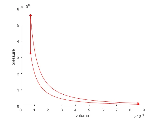
• This is the final plot of the Otto cycle. As the Otto cycle is not a standard cycle we will be having these types of curves. We can clearly see both the isentropic process and the constant volume heat addition and rejection process.

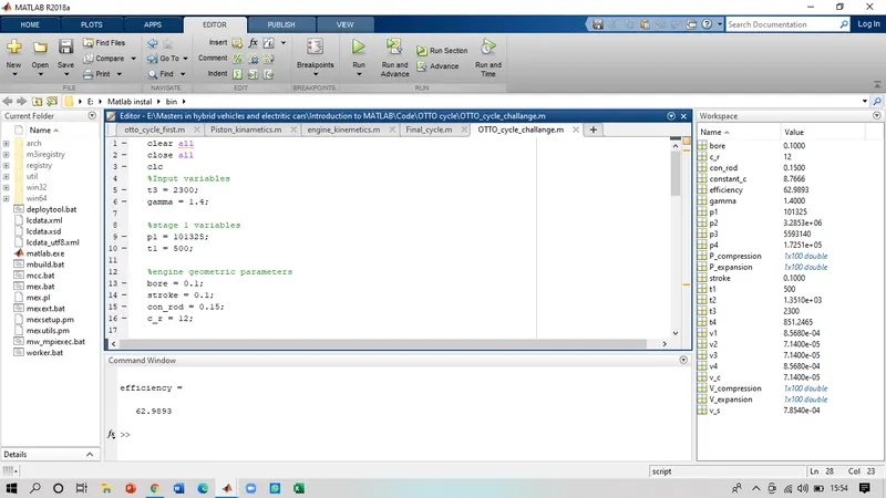
• The efficiency of the engine was calculated to be 62.98%, which was the output of the program.

ERRORS

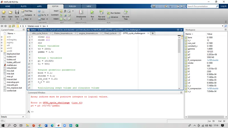
while writing the equation for pressure p4 missed the '*' sign in the equation, which created the above-mentioned error.

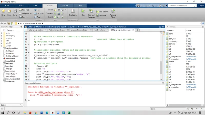
made a typing error while writing the plot command for the expansion plot.

CONCLUSION-

From the complete project, we can conclude that the code is suitable and is in working condition for computing the plot for an Otto cycle and its efficiency. By changing the parameters of the engine we can calculate the efficiency and plot an Otto cycle. For our engine, we receive a good efficiency of 62.98%. Using the same code and varying the geometric and engine parameters we can have a more efficient model as per requirement.