To Analysis TATA ULTRA T.16 TRUCK by equating various calculation and observing the ratio of Hill Climbing Power, Gradeability and To create Model for WOT (Wide Open Throttle) response of GM EV1 car.

AIM : To Analysis TATA ULTRA T.16 TRUCK by equating various calculation and observing the ratio of Hill Climbing Power, Gradeability and To create Model for WOT (Wide Open Throttle) response of GM EV1 car.

TATA T.16 ULTRA TRUCK :

Tata Motors Limited is India's largest automobile company and a market leader in the Country's commercial vehicles segment. As the world's fifth largest truck manufacturer, Tata Motors has crossed almost seven decades of automotive excellence in a journey marked with significant milestones in excellence and leadership. Using state-of-the-art technology in its world-class manufacturing units, the Company started exporting vehicles in 1961. Since then, Tata Motors has created a name globally, and completed 50 years of its international business in 2011.
Tata Motors was the first company to foray into the segment of indigenously developed Light Commercial Vehicles with the launch of Tata 407 and Tata 608 in 1986. Today, Tata Motors offers a wide range of light commercial vehicles (LCVs) and intermediate commercial vehicles (ICVs) widely used for inter-city and intra-city goods transport or passenger transport, with specific applications. Its range of revolutionary Light Trucks deliver superior performance, reliability and durability at low operating cost.

OBJECTIVE :

1. To find the ratio of hill climbing power required by fully loaded tata ultra truck to the half loaded one.
2. To find how much can be the minimum length of the flyover, considering the minimum height at the summit should be 5.5 meters.
3. To Prepare a new drive cycle excel file having third column representing hill climbing angle corresponding to speed and time. Revise the model file “Driver_Glider.slx” such that it can calculate gradient force from drive cycle.
4. Model the WOT (Wide Open Throttle) response of GM EV1 car. Compare it with the official figures of the performance of a real vehicle. Prepare a table showing variation in acceleration time with 5% change in vehicle parameters.

STUDY - 1 :

• To find the ratio of hill climbing power required by fully loaded tata ultra truck to the half loaded one.

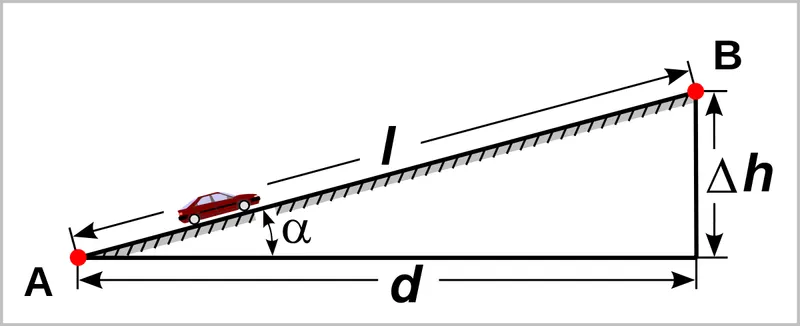
GIVEN DATA :

TATA T.16 Ultra Day Truck was considered for calculations. The specifications of the vehicle is as shown below :

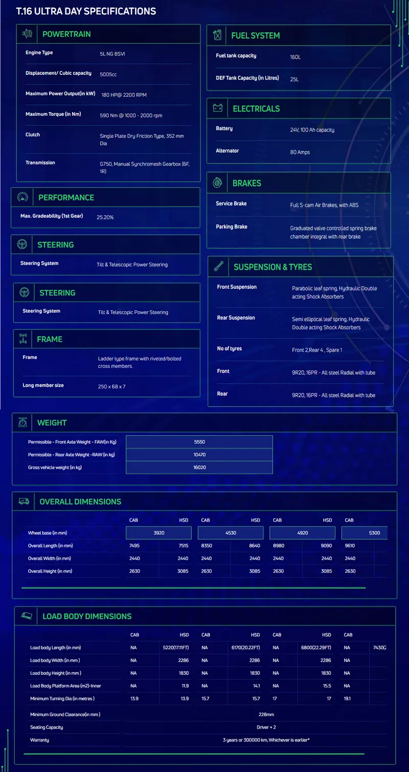
FORMULA USED :

HILL CLIMBING FORCE :

Fhc = m x g x sin(θ)

Where, m = Total mass

g = Gravity

POWER :

Power is a rate at which work is done, or energy is used. It is equal to the amount of work done divided by the time it takes to do the work. The unit of power is the Watt (W), which is equal to a Joule per second (J/s).

Total Power (P) = Total force (Fhc) x Speed (V)

Solution :

1. Calculation for Full loaded Truck :

   Vehicle kerb weight (kg) = 5550
   Vehicle payload weight (kg) = 10470

   Gross Vehicle weight (kg) = Vehicle kerb weight + Vehicle payload weight

   = 5550 + 10470

   = 16020

   Speed (V) = 35km/hr = 9.72 m/s

   Gradeability (θ) = 25.20% = 14.38°

   gravity (m/s^2) = 9.8
   

   As we know, the hill climbing force (Fhc) is given by :

   Fhc = m x g x sin(θ)

   = 16020 x 9.8 x sin (14.38°)

   = 38990.23N

   Now total power required (P) is given by :

   P = Fhc x V

   = 38990.23 x 9.72

   = 378985.03W

2. Calculation for Half loaded Truck :

   Vehicle kerb weight (kg) = 5550
   Vehicle payload weight (kg) = 10470/2 = 5235

   Gross Vehicle weight (kg) = Vehicle kerb weight + Vehicle payload weight

   = 5550 + 5235

   = 10785

   Speed (V) = 35km/hr = 9.72 m/s

   Gradeability (θ) = 25.20% = 14.38°

   gravity (m/s^2) = 9.8

   As we know, the hill climbing force (Fhc) is given by :

   Fhc = m x g x sin(θ)

   = 10785 x 9.8 x sin (14.38°)

   = 26249.04N

   Now total power required (P) is given by :

   P = Fhc x V

   = 26249.04 x 9.72

   = 255140.66W

Now, the ratio of full loaded vs half loaded :

Ratio = Full loaded Truck / Half loaded Truck

= 378985.03 / 255140.66

= 1.48

Therefore, the ratio is 1.48 .

STUDY - 2 :

• To find how much can be the minimum length of the flyover, considering the minimum height at the summit should be 5.5 meters.

Gradeability :

The grade (also called slope, incline, gradient, mainfall, pitch or rise) of a physical feature, landform or constructed line refers to the tangent of the angle of that surface to the horizontal. It is a special case of the slope, where zero indicates horizontality. A larger number indicates higher or steeper degree of "tilt". Often slope is calculated as a ratio of "rise" to "run", or as a fraction ("rise over run") in which run is the horizontal distance (not the distance along the slope) and rise is the vertical distance.

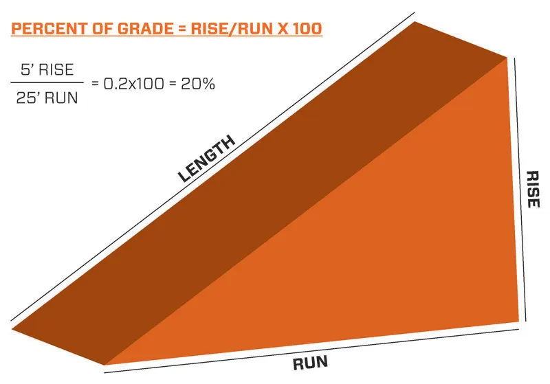
GIVEN DATA :

Minimum height = 5.5m

FORMULA USED :

GRADEABILITY :

Percentage of gradeability = ( Rise / Run ) x 100

PYTHAGORAS THEOREM :

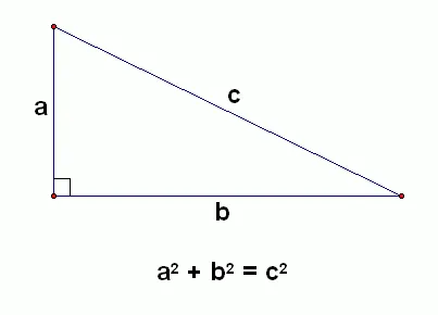
Rise² + Run² = Length²

Solution :

1. Calculation for Minimum Run of the flyover :

   Gradeability (θ) = 25.20%

   Minimum height (Rise) = 5.5m

   Percentage of gradeability = ( Rise / Run ) x 100

   Run = ( Rise / Percentage of gradeability ) x 100

   = ( 5.5 /25.20 ) x 100

   = 21.82m

   Minimum Run of the flyover is 21.82 meters .

2. Calculation for Minimum Length of the flyover :

Gradeability (θ) = 25.20%

Minimum height (Rise) = 5.5m

Minimum distance (Run) = 21.82m

Length² = Rise² + Run²

Length = √( Rise² + Run² )

= √( 5.5² + 21.82² )

= √(506.36)

= 22.50

Minimum Length of the flyover 22.50 meters

STUDY - 3 :

• To Prepare a new drive cycle excel file having third column representing hill climbing angle corresponding to speed and time. Revise the model file “Driver_Glider.slx” such that it can calculate gradient force from drive cycle.

DRIVER GLINDER SIMULINK MODEL :

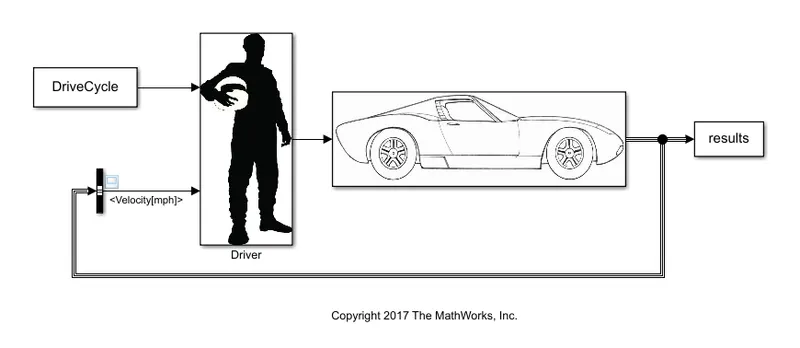
• In driver glider the velocity are assigned in excel sheet to find an acceleration of vehicle. The inputs values are plotted by graph as time and velocity.
• The unit conversion for veloicity is initiate in the new table and that value is taken as input of velocity.
• A speed of vehicle is varies with acceleration changes that will be calculated by time.
• Data's are inserted in MATLAB and that values are intiate in the velocity block to plot the acceleration of vehicle.

EXCEL SHEET FOR NEW DRIVE CYCLE :

Here the input values are assigned and entered in excel sheet. Time and velocity are assumed that data are inserted in driver
glider.

https://drive.google.com/file/d/1Hf5bWA7pR0w3ZYI5_xR-VzzV2q83N_2v/view?usp=sharing

NEW DRIVE CYCLE INPUT :

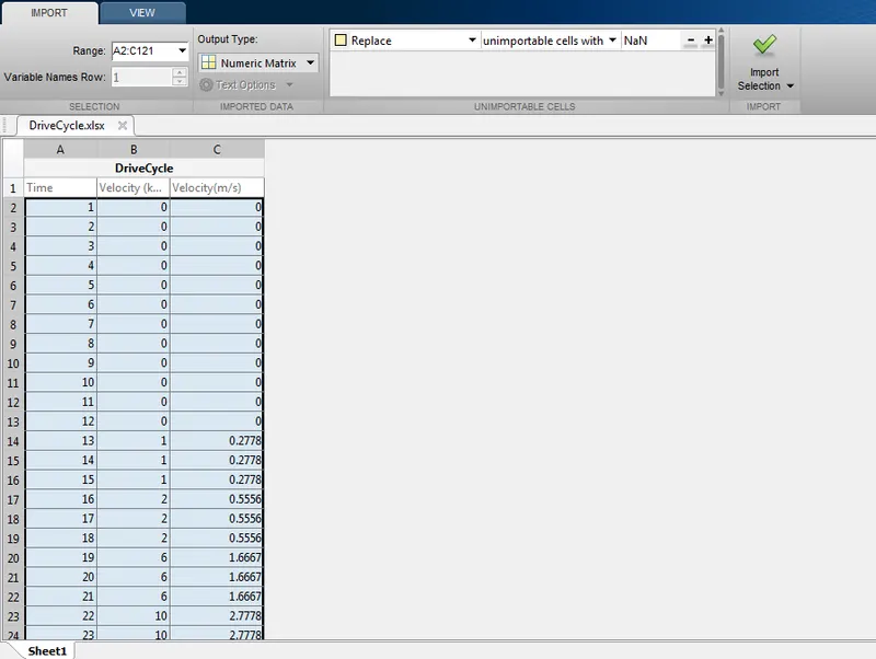
• The values of the drive cycle were then exported into Matlab workspace by selecting only the Time and Velocity m/s values, converting them into numerical values from the top “Output Type” selection.

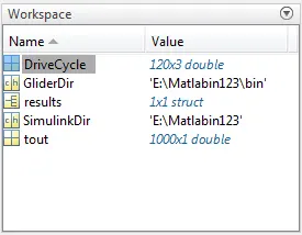
WORKSPACE AFTER IMPORTING SHEET :

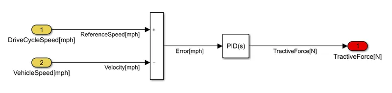
DRIVER SUBSYSYTRM :

GLINDER SUBSYSYTRM :

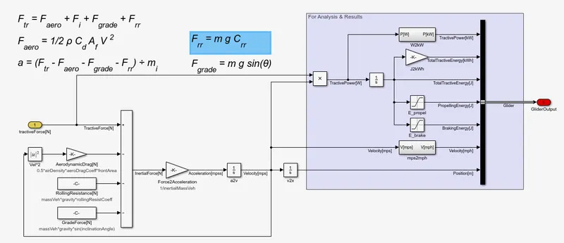
GRADIENT FORCE FROM DRIVE CYCLE :

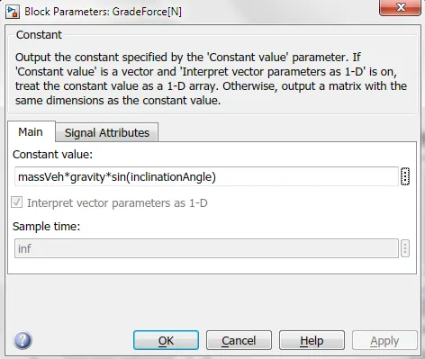
OUTPUT VELOCITY PLOTS :

WHEN INCLINATION ANGLE IS 0° :

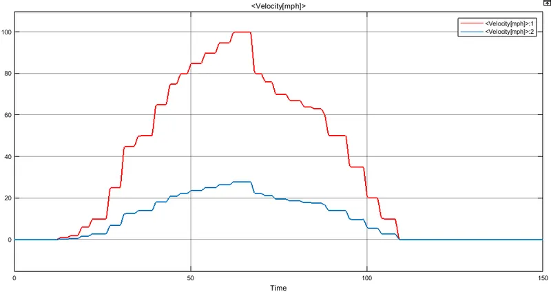
• Here, x-axis represents the time and y-axis represents the vehicle speed. We can see that, the vehicle considers only aerodynamic force and rolling resistance force, as the grade is 0.

WHEN INCLINATION ANGLE IS 40° :

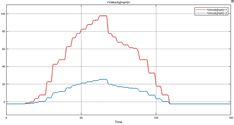
• As the inclination angle increases, there is more force required by the vehicle to overcome the grade. Here we can see that, the top speed reached is lesser than 100kmph, where as at 0 grade angle, the top speed goes to 100kmph according to the drive cyce.

STUDY - 4 :

• Model the WOT (Wide Open Throttle) response of GM EV1 car. Compare it with the official figures of the performance of a real vehicle. Prepare a table showing variation in acceleration time with 5% change in vehicle parameters.

WIDE OPEN THROTTLE (WOT) :

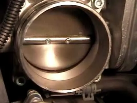
Wide open throttle or wide-open throttle (WOT), also called full throttle, is the fully opened state of a throttle on an engine (internal combustion engine or steam engine). The term also, by extension, usually refers to the maximum-speed state of running the engine, as the normal result of a fully opened throttle plate/butterfly valve. In an internal combustion engine, this state entails the maximum intake of air and fuel that occurs when the throttle plates inside the carburetor or throttle body are "wide open" (fully opened up), providing the least resistance to the incoming air.[1] In the case of an automobile, WOT is when the accelerator is depressed fully, sometimes referred to as "flooring it" (because automotive throttle controls are usually a pedal, so full throttle is selected by pressing the pedal to the floor, or as near as it will go). A throttle on a steam engine controls how much steam is sent to the cylinders from the boiler

CASE 1 :

Given GMEV Data :

Mass of vehicle = 1540kg

Drag Coefficient C = 0.19

Coefficient of rolling resistance µ = 0.0048

Angular velocity = 733 rad/s

Gear ratio = 11

Efficiency of drive = 0.95

Tyre radius = 0.3m

Critical velocity = 19.8 m/s

Motor torque = 140 Nm

Motor Speed = 12000 rpm

Constant Power = 102kW

Maximum velocity = 35.8 m/s

Calculations :

`T= 102000/(37*v)= 2756/v`

Also,

F = F + F + F + F

And `F= (T*G)/r`

Therefore,

`(T*G)/r= μ_rr*m*g+0.625AC_d v^2+(m+I G^2/(ƞ_g*r))* ((dv)/dt)`

Substituting and solving the given input values, we get :

`(dv)/dt=3.11-0.000137*v^2`

`(dv)/dt= 62.1/v-0.046-0.00317*v^2`

`v_(n+1)= v_n+ ∂t(3.11-0.000137v_n^2)`

`v_(n+1)= v_n+ ∂t(62.1/v_n -0.046-0.000137v_n^2)`

CODE :

clear all
close all
clc
t = linspace(0,20,201);
v = 0;
dt = 0.2;
for n = 1:200
 if v(n)<19.8
 v(n+1) = v(n)+ dt*(3.11-(0.000137*(v(n)^2)));
 elseif v(n)>=35.8
 v(n+1) = v(n);
 else
 v(n+1) = v(n)+ dt*((62.1/v(n))-0.046-(0.000137*(v(n)^2)));
 end
end
% Plotting
plot(t,v,'linewidth',2,'color','red');
xlabel("Time")
ylabel("Velocity")

Code Explaination :

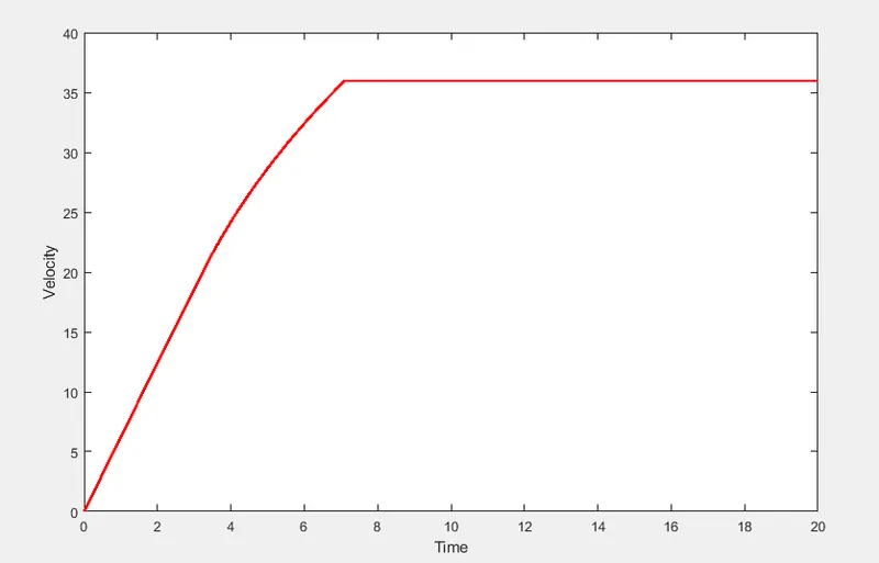
• The code contains a simple for loop in which there are three different conditions executed.
• The two equations which were obtained by calculations are used for two conditions i.e, when velocity is less than the critical value (velocity < 19.8 m/s) and for velocity beyond the maximum value (velocity >= 35.8 m/s). The third condition is when the velocity of the vehicle lies between 19.8 & 35.8 m/s.
• After executing it using "if-else" loop we finally plot the graph representing velocity vs time.

OUTPUT :

CASE 2 :

Changing the vehicle parameters by 5% :

Mass of vehicle = 1617kg

Drag Coefficient C = 0.1995

Coefficient of rolling resistance µ = 0.00504

Angular velocity = 769.65 rad/s

Gear ratio = 11

Efficiency of drive = 0.9975

Tyre radius = 0.315m

Critical velocity = 20.5 m/s

Motor torque = 147 Nm

Motor Speed = 12600 rpm

Constant Power = 107.1kW

Maximum velocity = 37.6 m/s

Solving for the above values, we get the following equations: -

`(dv)/dt=3.23-0.000152*v^2`

`(dv)/dt= 64.71/v-0.046-0.00152*v^2`

`v_(n+1)= v_n+ ∂t(3.23-0.000152v_n^2)`

`v_(n+1)= v_n+ ∂t(64.71/v_n -0.046-0.000152v_n^2)`

CODE :

clear all
close all
clc
t1 = linspace(0,20,201);
v1 = 0;
dt = 0.2;
for m = 1:200
 if v1(m)<20.5
 v1(m+1) = v1(m)+ dt*(3.23-(0.000152*(v1(m)^2)));
 elseif v1(m)>=37.6
 v1(m+1) = v1(m);
 else
 v1(m+1) = v1(m)+ dt*((64.71/v1(m))-0.046-(0.000152*(v1(m)^2)));
 end
end
% Plotting
plot(t1,v1,'linewidth',2,'color','blue');
xlabel("Time(sec)")
ylabel("Velocity(m/s)")
grid on

Code Explaination :

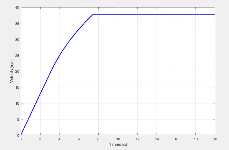
• The same process was followed as the previous code. The equations and values of velocities were changed due to 5% increase in the input parameters.

OUTPUT :

CASE 3 :

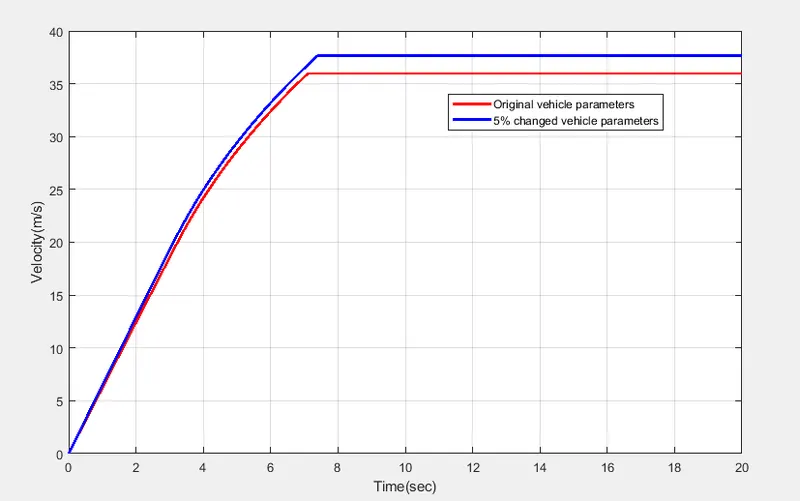
Comparing Both Outputs :

CODE :

clear all
close all
clc
t = linspace(0,20,201);
v = 0;
dt = 0.2;
for n = 1:200
 if v(n)<19.8
 v(n+1) = v(n)+ dt*(3.11-(0.000137*(v(n)^2)));
 elseif v(n)>=35.8
 v(n+1) = v(n);
 else
 v(n+1) = v(n)+ dt*((62.1/v(n))-0.046-(0.000137*(v(n)^2)));
 end
end
t1 = linspace(0,20,201);
v1 = 0;
dt = 0.2;
for m = 1:200
 if v1(m)<20.5
 v1(m+1) = v1(m)+ dt*(3.23-(0.000152*(v1(m)^2)));
 elseif v1(m)>=37.6
 v1(m+1) = v1(m);
 else
 v1(m+1) = v1(m)+ dt*((64.71/v1(m))-0.046-(0.000152*(v1(m)^2)));
 end
end
% Plotting
plot(t,v,'linewidth',2,'color','red');
hold on
plot(t1,v1,'linewidth',2,'color','blue');
xlabel("Time(sec)")
ylabel("Velocity(m/s)")
grid on
legend('Original vehicle parameters','5% changed vehicle parameters')

OUTPUT :

CONCLUSIONS :

Thus we have sucessfully answered all the questions in this challenge with proper outputs and matlab code.