The Law of Large Numbers and The Central Limit using Python

The Law of Large Numbers :

This is an important theorem in Statistics common to all of statistical inference and machine learning.

Example:

What is the average height of Canadians?

There are 40 mil people. So we cannot measure each and every single person. It is simply Not feasible.

So we instead draw a sample of say 50 people in Canada and measure their heights and then we take the average of that. This is the sample mean and not the population mean.

Question is how close the sample mean is to the population mean because the population mean is what we want to know.

Can we infer something about the relationship between sample mean and population mean?

From the Law of Large Numbers: in our examples where we take 50 random Canadians for Average Height

It states that if we get more and more groups of 50 randomly selected people, the average height of those groups will start to get closer and closer to the true population mean.

In other words, increasing the number of samples that we randomly select and take the sample mean of, the mean of these samples will get closer and closer to the ture mean of the whole data set.

For easier explaination:

the mean of the sample means will get more closer to the actual mean of the whole data set if we increase the number of samples that we take. So increase the number of samples then the mean of the Sample means will be closer to the actual Population Mean.

Mathematically we can say that if we take infinite samples then the

`=>"Mean of the sample means "= "Population mean"`

So in our case, it means that we dont have to measure the Height of each and every Canadian but just take a bunch of samples to get an approximately correct result of the Average Height of the 40 Million Canadians.

The Law of Large Numbers:

as the number of Experiments repitition increases, the Average of the Sample means better approximates the Population mean.

`=> lim_(n->oo)P(|barx_n - mu |> epsilon) = 0`

where `mu`= population mean or the true mean

`bar x` = sample mean of the sample chosen

`epsilon` = sribitrary small number greater than 0

n = number of samples taken

Interpretaion of the formula:

probability of the divergence between the sample mean and the population mean is a very small positive number (`epsilon`)

and that this small value of Divergence goes oto 0 if the number of samples(n) increase to an infinite number.

Why is the Law inportant in Statistics?

This is because any one sample is sensitive to many things such as sampling variability , noise and other non -systemic variations.

which means that one sample or one experiment is unlikely to provide a good estimate of the True Population mean. But sampling many times can help us get cloase to the True Population mean.

In our example:

Means that one sample/experiment is not going to be very trustworthy, that is , if we pick 50 canadians randomly their average height may not really reflect the true underlying height of the 40 mil people in Canada.

However by this law we can take a bunch of samples and more samples we take the more closer we get to the true mean.

implementation in Python

Steps of implementation:

step 1:

generate a population of numbers

we have to generate a bunch of numbers(population) and assign each member of the population a particular value(the height). we dont need to simulate too many numbers we will generate a couple 100 thousand numbers.

we will assign values according to 1/f shape, a 1/f distribution.

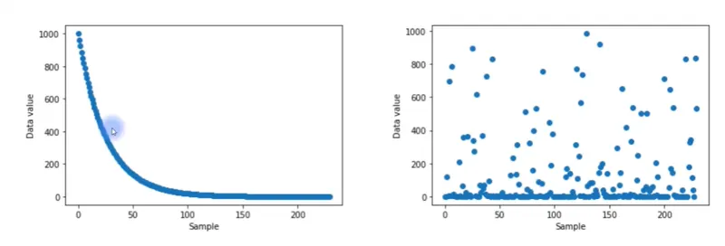
fig: Generation of Population with a 1/f distribution, then shuffling them to remove any instrinsic pattern

because we want to randomly generate the samples we have to sure that the numbers are randomly distributed. so we will generate the numbers like on the left graph but then shuffle/scramble all these numbers randomly so that there is no intrinsic ordering in the individual samnple points.

we will generate 230,000 points but it is not feasible to plot them on the graph, so the graph we see is actually 1 point after skipping 1000 samples , that is we have plotted every 1000th point.

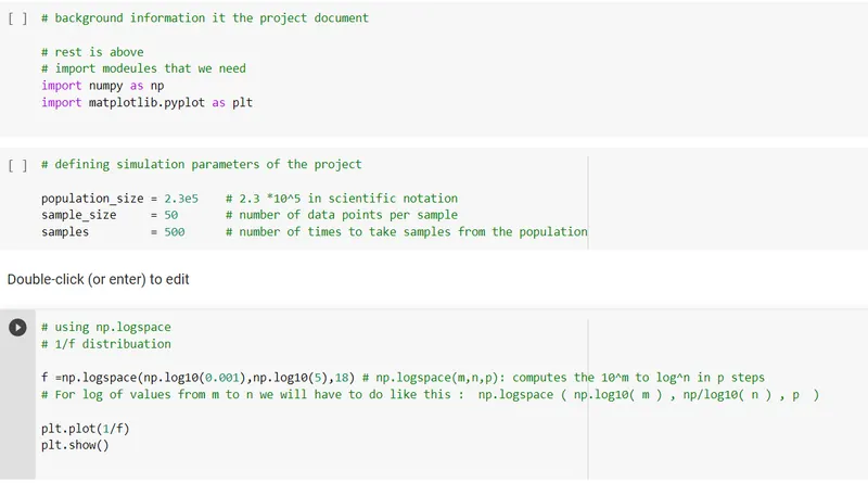
fig: code to generate and plot 1/f distribution for out popluation and plotting eavery 100th element

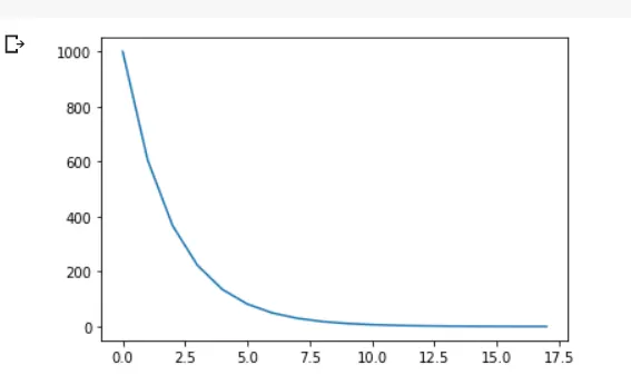
fig: Genearted form to shoe the 1/f distribution for of our population

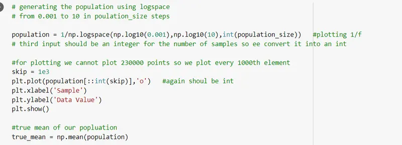
Fig: genearting the poplution for 2,30,000 people in a 1/f distribution

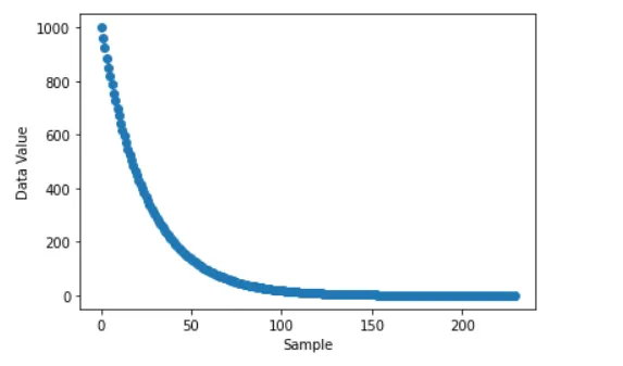
Fig: generated Popluation from the code above

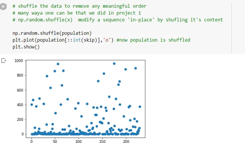
Fig: code to Shuffle the data to remove intrinsic patterns so that when we select 50 random values they are not following the 1/f pattern from which the data was produced

step 2:

Monte Carlo Sampling: it is nothing but selevting totally random data points from the population to find the mean of.

we will take 50 data points in each sample and 500 total samples.

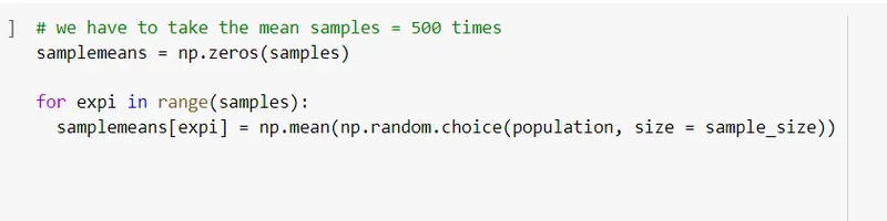
Fig: using np.random.choice(a,size =b) and finding the mean of each sample. Storing the mean of 500 samples in the variable 'samplemeans'

Now we will plot the means of All the 500 samples that we took from the population and also the Ture mean of the 230000 data points in out data set.

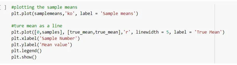
Fig: plotting the 500 sample means and True mean of the Data set

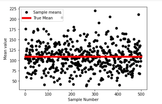
Fig: result of the code ton plot 500 Sample means and True mean of the Dataset

Discussion of the plot:

We see sometimes the sample mean of a sample is close to the true mean of the Data but sometimes they are very far away from each other, so from this we can see that individual samples are not reliable because the variability is too high

so according to the law of large number says it that :

the mean of the cloud of black dots together is going to be really close to the True Mean and the more of these samples we take, the more closer to the true mean we will get.

Step 3: Takling the Cumulative Average of the Sample means

it means that this: first point is taken is as itself 2nd point is replaced by the avergae of the 1st 2 data points 3rd point is replaced by the avergae of the 1st 3 data points 4th point is replaced by the avergae of the 1st 4 data points

and so on...

this will get much much closer to the true mean of the population compared to the indicidual sample means

This will slowly converge to the true mean.

what we expect is : the divergence of the cumulative averages and the true mean is decreasing as the number of samples is increasing. Sometimes it is positive and sometimes negative. Don't really care about the sign but the size of it.

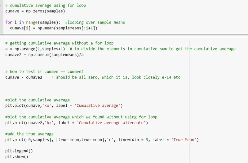
Fig: calculation of Cumulative average oin 2 ways : with and awithout for loop. and Plotting of both

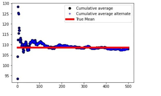
Fig: Result of the plot of the Cumualtive Average of the samples and the true mean

Discussion of th plot:

as expected , we see that the divergence of the Cumulative Average of the Sample means is Greater in the start. But as the number of Samples increase the diffference in the True mean and the Cumulative Average mean keeps on decreasing .

Which is what the Law of Large Numbers states. And Mathematically if number of samples (here 500) are increased to infinity then the difference in the Cumulative Average mean and the True mean will be 0.

Getting a closer look at the divergence with respect to the number of samples taken:

we know that the divergence will decrease as the number of smaples increase, also that it can be both positive and Negative

but we do not care about the sign of the divergence ,

So we will plot the Square of the divergence at each point of the 50 data points containing sample. And we will plot this for 100 samples.

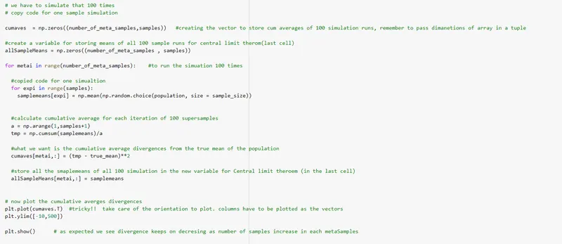
Fig: Code to implement the divergence Square at each of 50 points in a sample and plot it as a line. And repeating this process for 100 samples

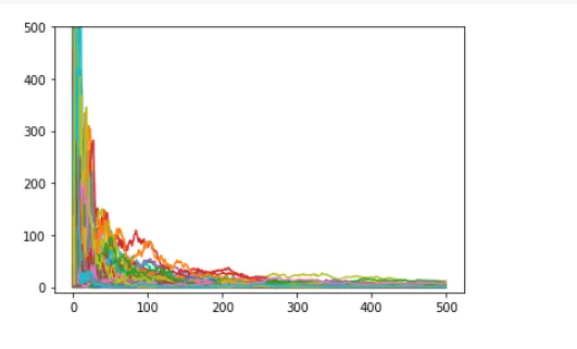
Fig: result of the above code.

Discussion of the plot: we see as expected that the divergence sqaure is highest in the start, but as the number of samples increase the divergence(difference in the Cumulative Average Sample mean ans the True mean) keeps on decreasing, this again proves the Law of large numbers.

Since we did the experiment 100 times we see that the law still holds true.

Step 4: The central limit theorem

The Central Limit Theorem: Central limit theorem tells use that the distribution of the sample means is going to be roughly gaussian distributed

The 2 theorems:

The law of large numbers tells that the sample means will be distributed around the True mean

And the central limit theorem tells us that the shape of that distribution will be gaussian in nature.

Process:

we will take 100 Meta samples, that is we did one experiment which had 500 samples with each sample having 50 randomly selected data points and then we found out the mean of the 500 Samples means anc compared it to the true mean

we will do this experiment 100 times

Consider one experiment result: from our last processing

Fig: plotting the 500 sample means from one experiment

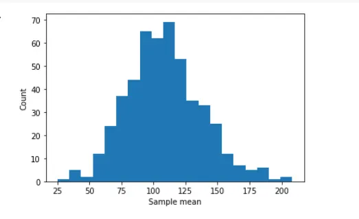
Fig: result of the plot . We see that the distribution of the sample means is Roughly Gaussian in nature. This is of 1 experiment

now we wwant to do 100 such experiments and plot the Histogram of each Sample means vector from each experiment as a line

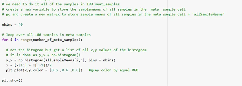
Fig: Code to plot the Histogram of Sample means for 100 experiment as a grey line

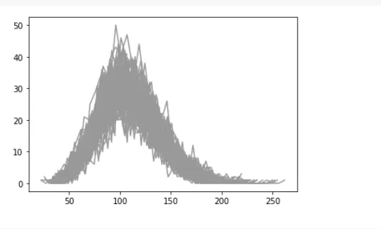
Fig: ressult of the Plots of 100 experiments

Discussion of the PLot: Central limit theorem proved: as we see that in 100 experiments ,the distribution of the 500 sample means in each experiment is Roughly Gaussian in nature.