Supervised Learning - Prediction Week 3 Challenge

Ans 1) Aim: To perform gradient descent in Python with any loss function:

Objective: To perform gradient descent in Python using mean square as a loss function on the following data set:

y= [1,2,3,4,5]

x=[0,1,2,3,4]

Theory:

J = (1/n)∑(y(i)-(mx(i) +b))², where

x(i) are the input

m and b are the weights

mx(i)+b is the predicted output and y(i) is actual value

Differentiating the loss function J with respect to m and b, we get

dJ/dm = (2/n)


∑−x(i)(y(i)−(mx(i)+b))

dJ/db = (2/n) ∑ - (y(i) - (mx(i) +b))

m and b values are then optimized

m = m -alpha*dJ/dm

b= b- alpha*dJ/db

alpha is the learning rate, i.e. how large a step the gradient takes.

Python code:

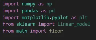
import numpy as np
import pandas as pd
import matplotlib.pyplot as plt
from sklearn import linear_model
from math import floor

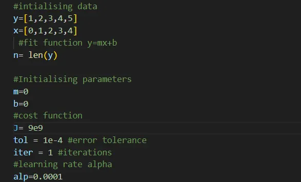
#intialising data
y=[1,2,3,4,5]
x=[0,1,2,3,4]
 #fit function y=mx+b
n= len(y)

#Initialising parameters
m=0
b=0
#cost function
J= 9e9
tol = 1e-4 #error tolerance
iter = 1 #iterations
#learning rate alpha
alp=0.0001
while(J>tol): #if error is greater than tolerance while loop is executed
    term1 =[]; #Empty array intialised
    d_m=[]; #Gradient of parameter m
    d_b=[];#Gradient of parameter b
    for i in range(0,n):
            term1.append(pow(y[i]-m*x[i]-b,2))
            d_m.append(-x[i]*(y[i]-m*x[i]-b))
            d_b.append(-y[i]+m*x[i]+b)
    print("\nNumber of iterations:",iter)
    iter = iter+1
    J = (1/n)*sum(term1)
    print("\nError:",J)
    print("\nParameters:")
    print("\nm value:",m)
    print("\nb value:",b)
    m = m- alp*(2/n)*sum(d_m)
    b = b- alp*(2/n)*sum(d_b)

Code explanation:

Necessary libraries are imported to execute the program:

Initial data and parameters are initialized:

Main body:

If condition J>tol is true, then the while loop will be executed.

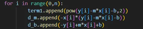
Inside the while loop, there is a for loop which fetches each value present in x and y and calculates the error and changes in the loss function for parameters m and b

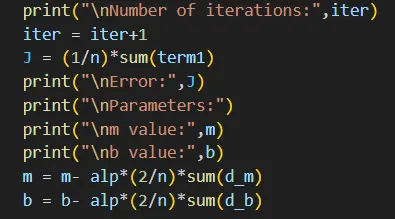
Output:

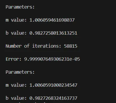
For a learning rate of 0.0001, it is concluded that for m value 1.006 and b value 0.9827 after the number of iterations 58815 the error could be lesser than the tolerance value.

Ans 2) Differences between L1 and L2 are :

L1 Mean absolute error:

Definition: find the mean of the absolute difference between the predicted and the actual value.

Calculation: It sums up the absolute difference between predictions and actuals and then averages them across the dataset.

Formula :

MAE= (1/n)Σ|y_i - ȳ|

where:

• (n) is the no. of data points.
• (y_i) represents the actual value.
• ȳ represents the predicted value.

Interpretation: MAE provides an easily interpretable error value because it is in the same scale as the target variable. It measures the magnitude of errors without considering their direction.

2. MSE(Mean squared error):

Definition: Finds the mean of the square of the differences between the predicted and actual value.

Calculations: It squares the differences between predictions and actual, sums them up and averages across the dataset. It is good for data sets with outliers, however, it returns an error in different units. Due to its mathematical properties, it is easier to calculate the gradients of the parameters.

Formula:

MSE = (1/n)Σ(y_i - ȳ)²

Interpretation: The squaring means that larger mistakes result in more errors than smaller mistakes, meaning that the model is punished for making the larger mistakes.

Finding the root mean squared error,i.e. using root mean square error brings the error term to match with the data set in terms of units.

Ans 3) Different loss functions used for regression are as follows:

1) Mean Squared Error(MSE):

• Also known as quadratic loss or L2 loss.
• Defined as the average of squared differences between the actual and predicted values.
• Mathematically, it can be expressed as:

MSE = (1/n)Σ(y_i - ȳ)²

where:

• (n) is the no. of data points.
• (y_i) represents the actual value.
• ȳ represents the predicted value.

2) Mean absolute Error(MAE):

• Also known as L1 loss.
• Measures the average differences between actual and predicted values.
• Mathematically, it can be expressed as:
• MAE= (1/n)Σ|y_i - ȳ|

3) Huber Loss(Smooth Mean Absolute Error):

• A robust loss function that combines the benefit of both MSE and MAE.
• It behaves like MAE for small errors and like MSE for large errors.
• Mathematically, it is defined as:

4) Log-Cosh Loss:

• A smooth approximation of Huber loss
• It is less sensitive to outliers than MSE.
• Mathematically, it can be expressed as:

Ans4) Let F be a function that determines the error between the data set and the predicted values. The predicted values depend on two parameters m and c. Gradient descent is a method to determine the values of the parameters for which F returns the least value.

Learning rate is an important factor that determines how fast the function parameter approaches a nominal value. Gradient descent is a method to determine the values of the function parameters for which the function returns the minimum error.

F = 1/(2n)*∑ⁿ_i=1 ((mx_i+c)- Y_i)²

m= m- α(∂F/∂m)

c= c- α(∂F/∂c)

Giving the high learning rate will cause the function to overshoot beyond its lowest value and will never reach its lowest value or oscillate before arriving at one.

Giving a lower learning rate will cause the function to approach the lowest value very slowly leading to a high number of iterations.

Ans 5) Linear regression can be evaluated by determining how good the fit is, i.e. what is the error between the predicted value and the data set.

R-Squared:

Assume the function f(x) to satisfy the data points (x1,y1),(x2,y2)...and so on.

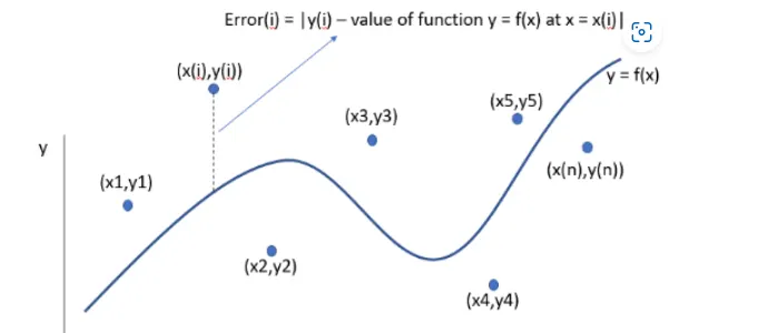
Sum of squared error SSE= ∑ⁿ_i=1(y(i)-f(x(i)))²

If the proposed equation is an nth-degree polynomial

f(x) = A1+A2.x+A3.x²+..+A_n.x^n-1

Differentiating the SSE with each coefficient and equating it to zero will return us the value of the coefficient for which the error is minimum.

solving the multiple systems of equations we can get the value of coefficients. This is the least square error method.

R-square:

R square =SSR/SST, where

SST = SSE+SSR

SSR stands for the sum of the squares of the regression and is equal to the square of the difference between the value of the fitting function at the given point and the mean of the data set.

SSR stands for the sum of the squares of the regression and is equal to the square of the difference between the value of the fitting function at the given point and the mean of the data set.

SSR = ∑ⁿ_i=1(f(x(i) - M)², where M is the arithmetic mean of the given data set.

Ans 6) Difference between multiple and adjusted coefficients of determination:

when the dependent variable depends on only one independent variable then it is known as the linear coefficient of determination, but when it depends on multiple independent variables then it is the multiple coefficient of determination.

The adjusted coefficient of determination is a method in which the parameters that do not contribute towards the predicted value are ignored. These parameters are called insignificant independent variables.

Adding new variables to the system will affect the R-squared value and the adjusted R-squared disregards the infinitesimally small increments and only considers the parameters which contribute to the output in a significant way

R²_adj = 1 - (1-R²)(n-1)/(n-k-1), where

n = number of data points

k = number of independent variables

Case 1: If added variables are insignificant, that means k will increase with little or no effect on R^2_, hence R²_adj will decrease.

Case 2: If added variables are significant, that means k will increase with a significant increase in R², hence R²_adj will also increase.