Supervised Learning - Classification Week 8 Challenge
1. Pros and cons of knn
ADVANTAGES
i, K-NN is pretty intuitive and simple
ii, K-NN has no assumptions.ie, it is a non-parameteric algorithm.
iii, No training step - does not require indiviudal training to the model and so called Lazy learning model
iv,It constantly evolves - it is a memory based approach and respond quickly to the changes in the input.
v, Very easy to implement for multi-class problem
vi, can be used for both classification and regression problem.
vii, Only one-hyper parameter
viii, Giving flexibility to the users to choose between various distance algorithm.
1, Euclidian distance.
2, Hamming Distance
3, Manhattan Distance
4, Minkowski Distance
DISADVANTAGES:
1. K-NN might be easy, but as the dataset grows, efficiency or speed of the algorithm declines very fast
2. Curse of Dimensionality: KNN work well with small number of input variables, but as the numbers of variables grow K-NN algorithm struggles to predict the output of new data point
3. K-NN needs homogeneous features: The features should be standardized and normalized before using it in the function.
4. Choosing Optimal value of the Neighbors
5. Imbalanced dataset causes problems.
6. Outlier sensitivity and missing value treatment - it is very sensitive to outliers as it simply chooses the neighbors based on distance criteria. And it inherently has no capability of dealing with missing value problem.
1. Apply k-nn to the dataset
Given file:

COLAB - LINK
Modules used:
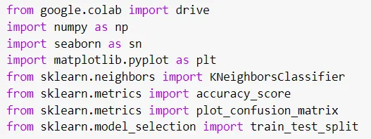
Step 1: To read the given data using pandas:
When the data is read, it is found that the last 7 columns were of categorical form with values 1 and 0. Hence last 7 columns will be asssigned as target and the remaining columns will be assigned as features.

df.head() command displays the first five rows and all the columns of the given data.
df.iloc[:,:27] assigns first 27 features to the variable X.
df.iloc[:,-7:] assigns last 7 features to the variable Y.
df.info() command displays all the rows and columns along with type of integer.
this command checks whether there are any empty columns and displays the output as true or false.
Step 2 : To filter the given data and the codes are explained in the image below
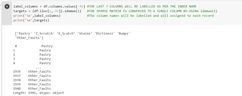
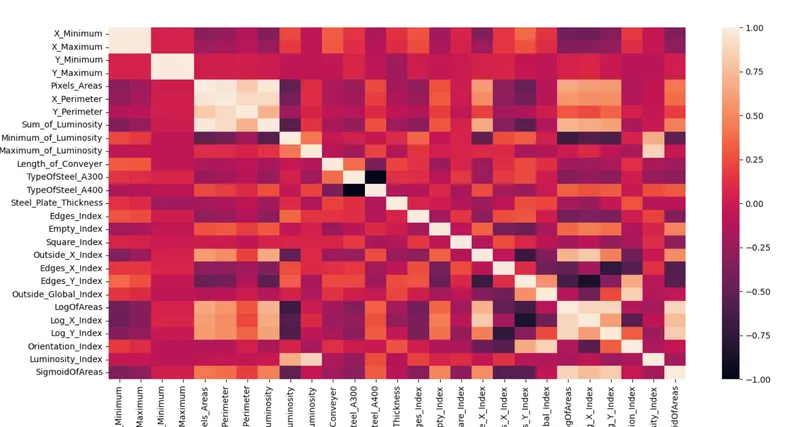
Step 3 : To find the correlation between the given features and to reduce the dimension of the feature, heat map is generated using seaborn module.
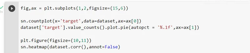
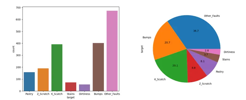
pie chart, bar graph for target variables and heatmap for feature variable are generated to find the correlation and reduce the dimension of the problem.
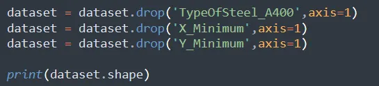
The features ('Typeofsteel_A400,X_MINIMUM and Y_MINIMUM') are dropped from the dataset using the above command.
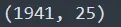
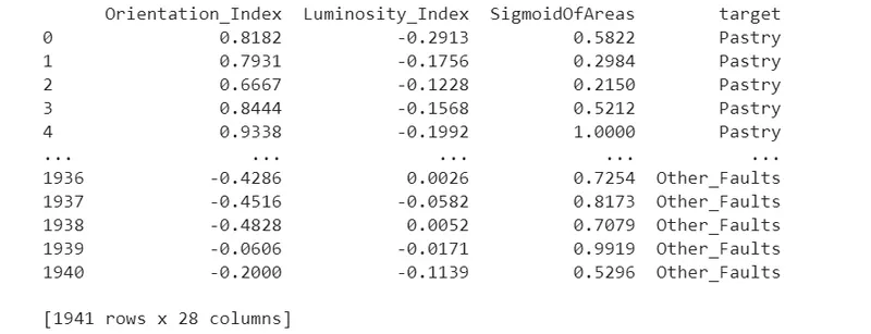
print(dataset.shape) shows the result after the dimension reduction.
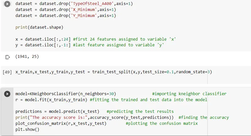
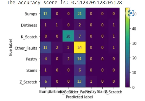
CONFUSION MATRIX AND ACCURACY SCORE FOR 90:10 DATA SET
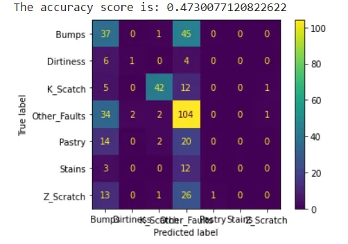
CONFUSION MATRIX AND ACCURACY SCORE FOR 80:20 DATA SET
CONFUSION MATRIX AND ACCURACY SCORE FOR 70:30 DATA SET
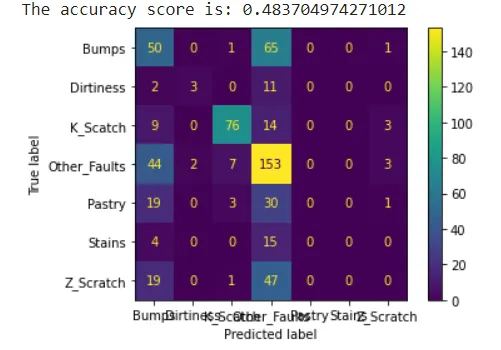
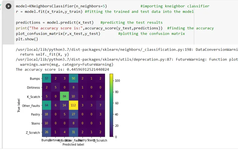
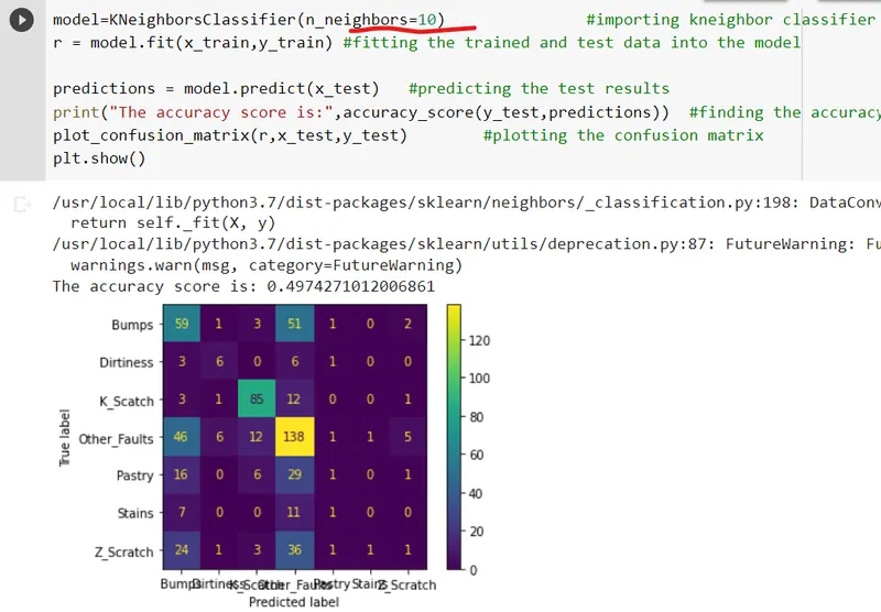
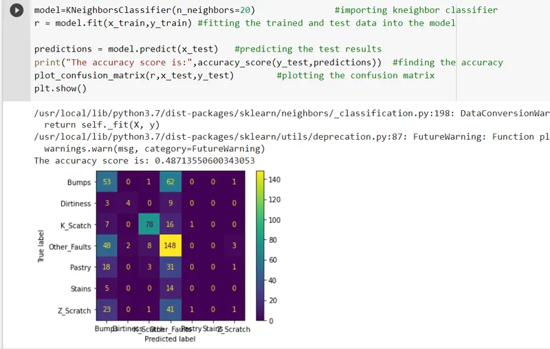
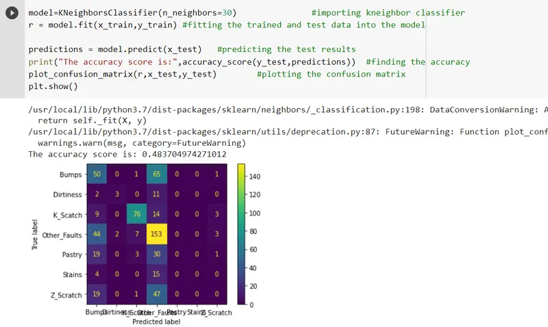
Observations: from the confusion matrix , it is very clear that there are many non-zero values along the non diagonal row of the matrix. Hence the accuracy will be very low (almost 50%) .
CONFUSION MATRIX AND ACCURACY SCORE FOR K=30 NN.20NN,10NN,5NN