Supervised Learning - Classification Week 7 Challenge

1. Pros and cons of SVM

PROS:

i, It works really well with a clear margin of seperation.

ii, It is effective in high dimensional spaces.

iii, It is effictive in cases where the number of dimensions are greater than the number of samples.

iv, It uses a subset of training points in the decision function (called support vectors), so it is also memory efficient.

CONS:

i, It doesn't peform well when we have large data set because the required training time is higher.

ii, It also doesn't perform very well, when the data set has more noise. i.e, target classes are overlapping

iii, SVM doesn't directly provide probability estimates, these are calculated using an expensive five-fold cross- validation.

2. Apply SVM to the “Surface defects in stainless steel plates” dataset and evaluate it

Given file:

PYTHON CODE:

import math
import pandas as pd
import matplotlib.pyplot as plt
import numpy as np
import seaborn as sn
from sklearn import svm
from sklearn.metrics import accuracy_score
from sklearn.metrics import plot_confusion_matrix
from sklearn.model_selection import train_test_split

df = pd.read_csv('faults.csv')
print(df.head())
X = df.iloc[:,:27]
Y = df.iloc[:,-7:]

print(df.isnull().values.any())

														
label_columns = df.columns.values[-7:] #THE LAST 7 COLUMNS WILL BE LABELLED AS PER THE INDEX NAME
targets = (df.iloc[:,-7:]).idxmax(1)   #THE SPARSE MATRIX IS CONVERTED TO A SINGLE COLUMN BU USING idxmax(1)
print('\n',label_columns)              #The column names will be labelled and will assigned to each record
print('\n',targets)

dataset = df.drop(label_columns,axis=1) #the dropped column dataset will be assigned to the variable 'dataset'
dataset['target'] = targets             #a new column named target will be assigned to the dataset along with other features
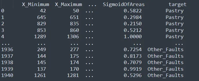
print('\n',dataset)

fig,ax = plt.subplots(1,2,figsize=(15,6))

sn.countplot(x='target',data=dataset,ax=ax[0])
dataset['target'].value_counts().plot.pie(autopct = '%.1f',ax=ax[1])

plt.figure(figsize=(10,11))
sn.heatmap(dataset.corr(),annot=False)

dataset = dataset.drop('TypeOfSteel_A400',axis=1)
dataset = dataset.drop('X_Minimum',axis=1)
dataset = dataset.drop('Y_Minimum',axis=1)

print(dataset.shape)

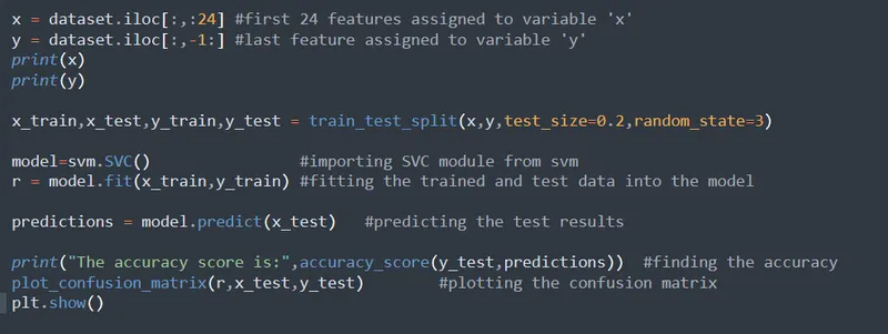
x = dataset.iloc[:,:24] #first 24 features assigned to variable 'x'
y = dataset.iloc[:,-1:] #last feature assigned to variable 'y'
print(x)
print(y)

x_train,x_test,y_train,y_test = train_test_split(x,y,test_size=0.2,random_state=3) 

model=svm.SVC()                #importing SVC module from svm
r = model.fit(x_train,y_train) #fitting the trained and test data into the model

predictions = model.predict(x_test)   #predicting the test results 

print("The accuracy score is:",accuracy_score(y_test,predictions))  #finding the accuracy
plot_confusion_matrix(r,x_test,y_test)        #plotting the confusion matrix
plt.show()  

Code snippets:

Modules used:

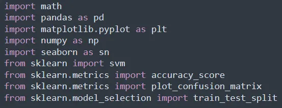
Step 1: To read the given data using pandas:

When the data is read, it is found that the last 7 columns were of categorical form with values 1 and 0. Hence last 7 columns will be asssigned as target and the remaining columns will be assigned as features.

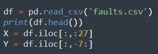
df.head() command displays the first five rows and all the columns of the given data.

df.iloc[:,:27] assigns first 27 features to the variable X.

df.iloc[:,-7:] assigns last 7 features to the variable Y.

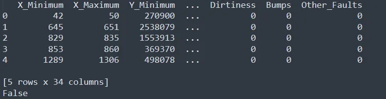
df.info() command displays all the rows and columns along with type of integer.

this command checks whether there are any empty columns and displays the output as true or false.

Step 2 : To filter the given data and the codes are explained in the image below

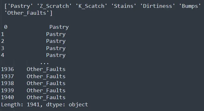
Step 3 : To find the correlation between the given features and to reduce the dimension of the feature, heat map is generated using seaborn module.

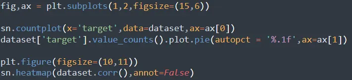
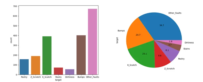
pie chart, bar graph for target variables and heatmap for feature variable are generated to find the correlation and reduce the dimension of the problem.

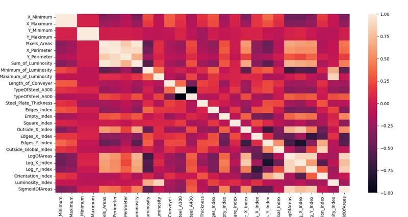
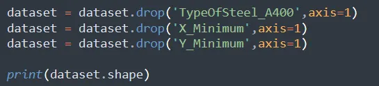
The features ('Typeofsteel_A400,X_MINIMUM and Y_MINIMUM') are dropped from the dataset using the above command.

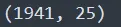
print(dataset.shape) shows the result after the dimension reduction.

CONFUSION MATRIX

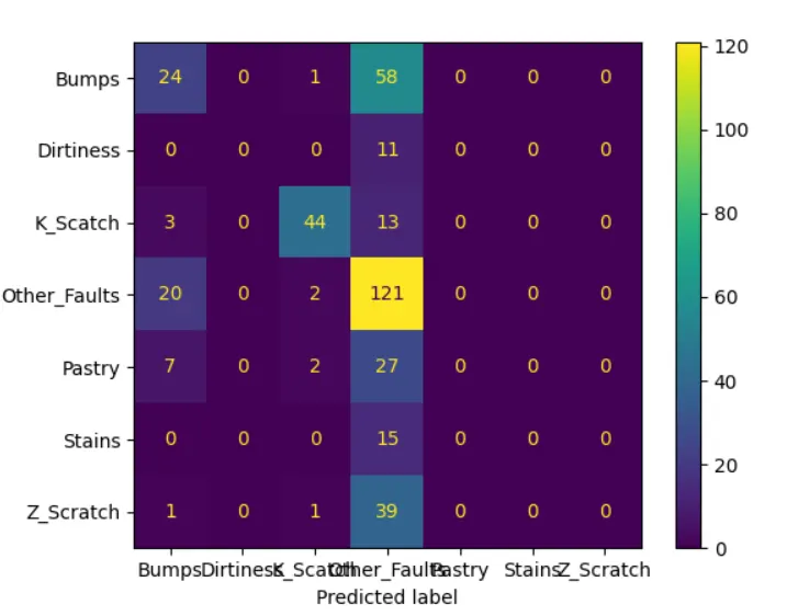
Observations: from the confusion matrix , it is very clear that there are many non-zero values along the non diagonal row of the matrix. Hence the accuracy will be very low (almost 50%) .