Supervised Learning - Classification Week 7 Challenge

1. Pros and cons of SVM

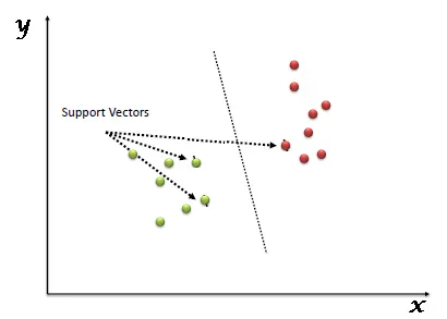
“Support Vector Machine” (SVM) is a supervised machine learning algorithm that can be used for both classification or regression challenges. However, it is mostly used in classification problems. In the SVM algorithm, we plot each data item as a point in n-dimensional space (where n is the number of features you have) with the value of each feature being the value of a particular coordinate. Then, we perform classification by finding the hyper-plane that differentiates the two classes very well (look at the below snapshot).

• Pros:
  • It works really well with a clear margin of separation
  • It is effective in high-dimensional spaces.
  • It is effective in cases where the number of dimensions is greater than the number of samples.
  • It uses a subset of training points in the decision function (called support vectors), so it is also memory efficient.
• Cons:
  • It doesn’t perform well when we have large data set because the required training time is higher
  • It also doesn’t perform very well, when the data set has more noise i.e. target classes are overlapping
  • SVM doesn’t directly provide probability estimates, these are calculated using an expensive five-fold cross-validation. It is included in the related SVC method of the Python scikit-learn library.

2. Apply SVM to the “Surface defects in stainless steel plates” dataset and evaluate it

import pandas as pd
import numpy as np
import seaborn as sns
import matplotlib.pyplot as plt

df=pd.read_csv("faults.csv")
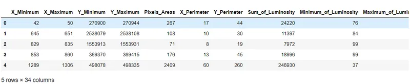
df.head()

df.isnull().sum()

df.info()

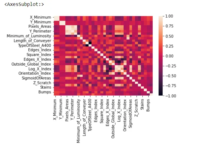
# Calculate correlations heatmap
corr = df.corr()
sns.heatmap(corr)

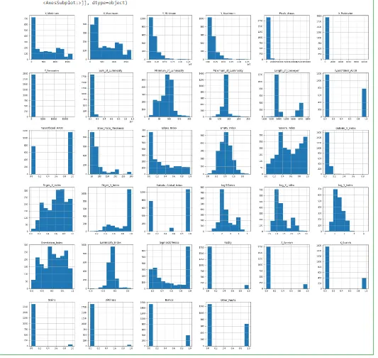
df.hist(figsize=(30,30))

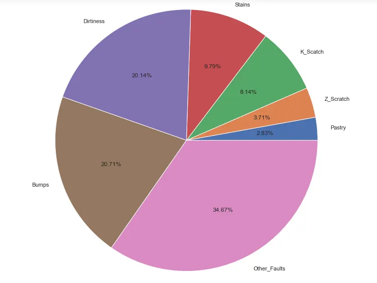
Faults = df[['Pastry', 'Z_Scratch', 'K_Scatch', 'Stains', 'Dirtiness', 'Bumps', 'Other_Faults']]
Attributes = df.drop(columns = Faults)

plt.subplots(figsize = ([12,12]))
plt.pie(x=Faults.value_counts().sort_values(),autopct = '%.2f%%',labels = Faults.columns)

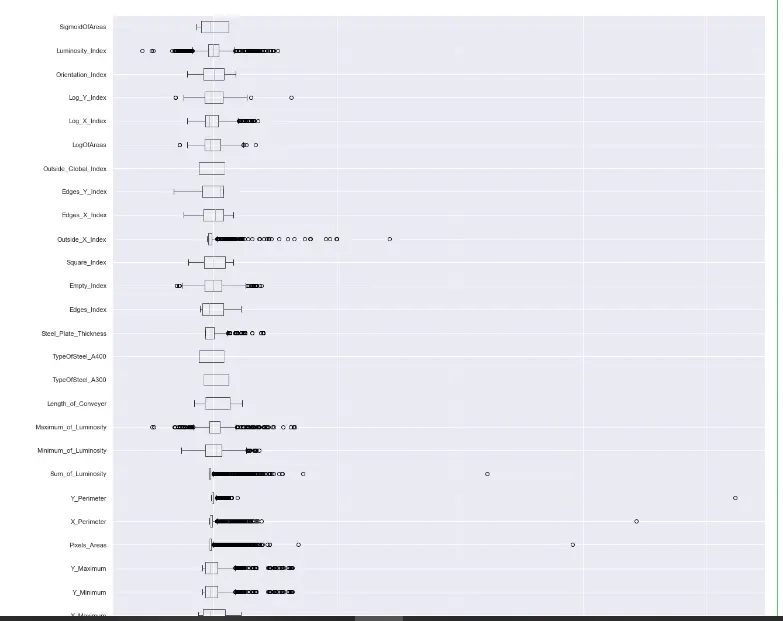
Standard Scaler:

from sklearn.preprocessing import StandardScaler
scaler = StandardScaler()
Attributes_scaled = pd.DataFrame(scaler.fit_transform(Attributes),columns = Attributes.columns)
Attributes_scaled.boxplot(return_type = 'axes',figsize = (20,20),vert = False)

Target = []
for i in range(Faults.shape[0]):
if df['Pastry'].values[i] == 1:
Target.append('Pastry')
elif df['Z_Scratch'].values[i] == 1:
Target.append('X_Scratch')
elif df['K_Scatch'].values[i] == 1:
Target.append('K_Scatch')
elif df['Stains'].values[i] == 1:
Target.append('Stains')
elif df['Dirtiness'].values[i] == 1:
Target.append('Dirtiness')
elif df['Bumps'].values[i] == 1:
Target.append('Bumps')
else:
Target.append('Other_Faults')

Target = pd.DataFrame(Target)
df['Target'] = Target

Splitting the data into training and test data:

from sklearn.model_selection import train_test_split

X_train,X_test,y_train,y_test = train_test_split(Attributes_scaled,Target,test_size = 0.3,random_state = 4)

Training SVM classification on training set:

from sklearn import svm
model = svm.SVC(C = 1,kernel = 'linear',gamma = 'auto')
fit_model = model.fit(X_train,y_train)

Predicting the score:

score = fit_model.score(X_test,y_test)
score

0.7341337907375644

Predicting the test results:

y_predict = fit_model.predict(X_test)
y_predict

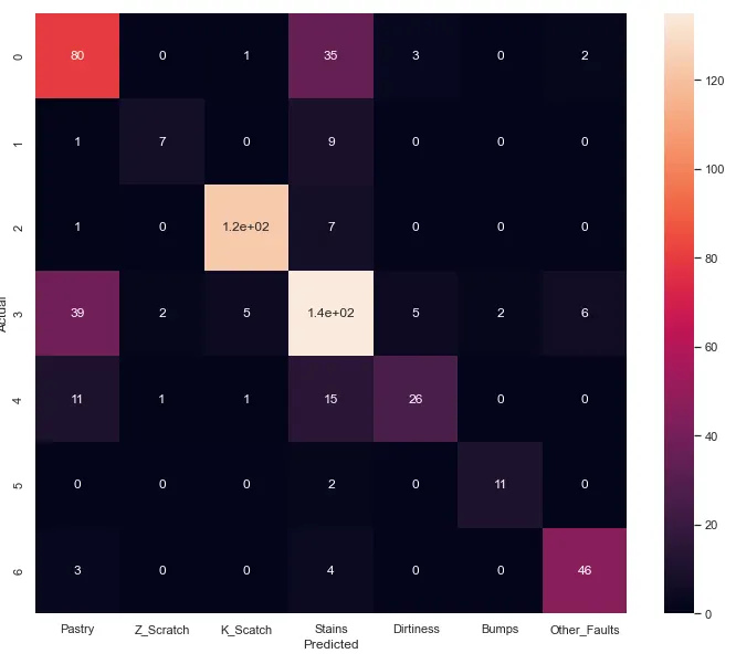
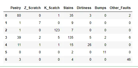
Confusion matrix:

from sklearn import metrics
cm = metrics.confusion_matrix(y_test,y_predict)
cm = pd.DataFrame(cm,columns = Faults.columns)
cm

Visualize confusion matrix through heat map:

sns.set(rc={'figure.figsize': (12,10)})
sns.heatmap(cm,annot=True)
plt.xlabel("Predicted")
plt.ylabel("Actual")
plt.show()