Genetic Algorithm

A genetic algorithm is a search-based optimization technique based on the principles of genetics and natural selection. It is frequently used to find optimal or near-optimal solutions.

we can apply the genetic algorithm that is not well suited for the standard optimization algorithm.

MATLAB ga calculates the minimum value of the inverted functions, so to find the global maximum function we can invert the function whose global max is to be found.

Firstly we will create our own function for x and y

Function:

function[F] = stalagmite(input_vector);
a = input_vector(1);
b = input_vector(2);
f1_x = [sin(5.1*pi*a + 0.5)]^6;
f1_y = [sin(5.1*pi*b + 0.5)]^6;
f2_x = exp(-4*log(2)*(((a-0.0667)^2)/0.64));
f2_y = exp(-4*log(2)*(((b-0.0667)^2)/0.64));
F = -(f1_x*f1_y*f2_x*f2_y);
end

We will name it as stalagmite function and save the file.

Then we will use linspace command to find various x and y values.

Then create a matrix using the meshgrid.

Now values in the different matrix can be put as an input into a function that we have created, then we get values of various values of function x and y.

Now we will use the for loop and then irate them into 50 times.

use syntax [inputs, fopt(i)]=ga(@stalagmite,2);

x = ga(fun,nvars)

In input we get 1*2 matrix for each iteration it will basically give the value of x and y.fopt will give the optimum values of the function at x and y.

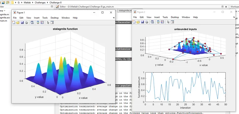
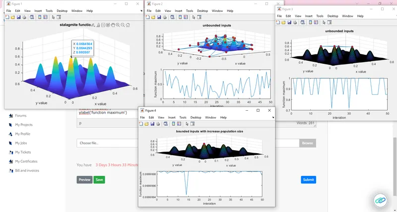
The inputs can be stored and surf command to create a surface to visualize the function.

We can also use the marker command to point to the local maximum.

Now for second syntax

x = ga(fun,nvars,A,b,Aeq,beq,lb,ub)

Since there is no inequal constraints or equal constraints A,b,Aeq,beq are represented as []

[inputs,fopt(i)]= ga(@stalagmite, 2, [], [], [],[], [0,0],[0.6,0.6])

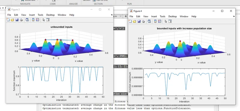
If we execute the loop we will get different local maxima with bounded inputs

now for 3rd syntax

x = ga(fun,nvars,A,b,Aeq,beq,lb,ub,nonlcon,options)

Since there is no inequal constraints or equal constraints A,b,Aeq,beq, nonlcon are represented as []

[inputs,fopt(i)]= ga(@stalagmite, 2, [], [], [],[], [0,0],[0.6,0.6],[],[],options);

This can help us to converge the most aqcurate solution

close all
clear all
clc
% defining our search space
x = linspace(0, 0.6, 150);
y = linspace(0, 0.6, 150);
num_cases = 50;

% creating 2 dimentional mesh
[XX,YY] = meshgrid(x,y);

%Evaluate stalagmite function
for i = 1:length(XX)
for j = 1:length(YY)
input_vector(1)=XX(i,j);
input_vector(2)=YY(i,j);
F(i,j)=stalagmite(input_vector);
end
end
figure(1)
surfc(XX,YY,-F)
shading interp
xlabel('x value')
ylabel('y value')
title('stalagmite function')

for i= 1:num_cases
[inputs, fopt(i)]=ga(@stalagmite,2);
xopt(i)=inputs(1);
yopt(i)=inputs(2);
end
figure(2)
subplot(2,1,1)
surfc(XX,YY,-F)
shading interp
title('unbounded inputs')
xlabel('x value')
ylabel('y value')

hold on
plot3(xopt,yopt,-fopt,'-o','markerfacecolor','r')
subplot(2,1,2)
plot(-fopt)
xlabel('interation')
ylabel('function maximum')

for i = 1:num_cases
[inputs,fopt(i)]= ga(@stalagmite, 2, [], [], [],[], [0,0],[0.6,0.6]);
xopt(i)=inputs(1);
yopt(i)=inputs(2);
end
figure(3)
subplot(2,1,1)
surfc(XX,YY,-F)
shading interp
title('unbounded inputs')
xlabel('x value')
ylabel('y value')
hold on

plot3(xopt,yopt,-fopt,'-o','markerfacecolor','r')
subplot(2,1,2)
plot(-fopt)

xlabel('interation')
ylabel('function maximum')

options = optimoptions(@ga)
options = optimoptions(@ga, 'populationsize', 250);

for i = 1:num_cases
[inputs,fopt(i)]= ga(@stalagmite, 2, [], [], [],[], [0,0],[0.6,0.6],[],[],options);
xopt(i)=inputs(1);
yopt(i)=inputs(2);
end
figure(4)
subplot(2,1,1)
surfc(XX,YY,-F)
shading interp
title('bounded inputs with increase population size')
xlabel('x value')
ylabel('y value')
hold on

plot3(xopt,yopt,-fopt,'-o','markerfacecolor','r')
subplot(2,1,2)
plot(-fopt)
xlabel('interation')
ylabel('function maximum')