Solving second order ODEs

Code:

clear all
close all
clc

b = 0.05;
g = 9.81;
l = 1;
m = 0.1;

% initial condition
theta_0 =[0;5];
% time points
t_span = linspace(0,10,250);

% solve ODE
[t, results] = ode45(@(t,theta) ode_func(t, theta, b, g, l, m), t_span, theta_0);

plot(t, results(:,1))
hold on
plot(t, results(:,2))
ylabel('plot')
xlabel('time')
title('for simple pendulum')

% animate pendulum

amplitude=results(:,1);
p=1;
for i=1:length(amplitude)
angle= amplitude(i);
figure(2)
title('simple pendulum')
% fix point of pendulum
x0=0;
y0=0;
% anoher end of pendulum/cordinate of mass ball
x1=l*sin(angle);
y1=-l*cos(angle);

%plot
plot([-1.1 1.1],[0,0],'linewidth',2);
hold on
plot([x0 x1],[y0,y1],'color','g','linewidth',2)
plot(x1,y1,'.','markersize',50)
hold off
grid on
axis([-2 2 -1 0])
pause(0.001)
M(p)=getframe(gcf);
p=p+1;
end
% making movie
movie(M)
videofile= VideoWriter('simple_pendulum1.avi');
open(videofile)
writeVideo(videofile,M)
close(videofile)

Function:

function [dtheta_dt] = ode_func(t,theta,b,g,l,m)

theta1 = theta(1);
theta2 =theta(2);
dtheta1_dt = theta2;
dtheta2_dt = -(b/m)*theta2 - (g/l)*sin(theta1);
dtheta_dt = [dtheta1_dt; dtheta2_dt];
end

Result:

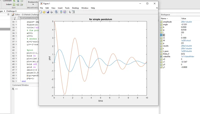
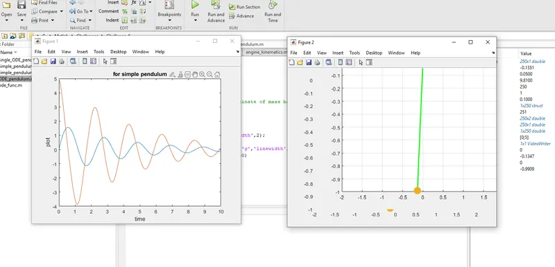
The graph shows time vs displacement(Blue) and time vs velocity(Red) the displacement is decreasing continuously due to the damping coefficient also angular velocity is in decreasing order.