Air standard Cycle
write code that can solve an otto cycle and make plots for it.
"""
otto cycle simulator
"""
import math
import matplotlib.pyplot as plt
#input
p1= 101325
t1= 500
gamma=1.4
t3=2300
#write code that can solve an otto cycle and make plots for it.
#geometric parametres
bore=0.1
stroke=0.1
con_rod=0.15
cr=12
#volume coputation
v_s = (math.pi/4)*pow(bore,2)*stroke
v_c = v_s/(cr-1)
v1 = v_s+v_c
#state point 2
v2=v_c
#p2v2^gamma = p1v1^gamma
p2 = p1*pow(v1,gamma)/pow(v2,gamma)
#p2v2/t2 = p1v1/t1 | p1v1/t1 = rhs | p2v2/t2 = rhs | t2 = p2v2/rhs
rhs = p1*v1/t1
t2 = p2*v2/rhs
#state point 3
v3=v2
#p3v3/t3 = p2v2/t2 | rhs = p2v2/t2 | p3 = rhs*t3/v3
rhs = p2*v2/t2
p3 = rhs*t3/v3
#state point 4
v4=v1
#p4v4^gamma = p3v3^gamma
p4 = p3*pow(v3,gamma)/pow(v4,gamma)
#p4v4/t4 = rhs
t4 = p4*v4/rhs
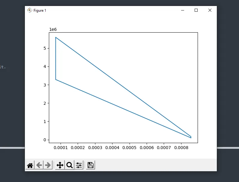
plt.plot([v1,v2,v3,v4,v1],[p1,p2,p3,p4,p1])
plt.show()
"""
otto cycle simulator
"""
import math
import matplotlib.pyplot as plt
def engine_kinematics(bore,stroke,con_rod,cr,start_crank,end_crank):
a = stroke/2
R =con_rod/a
#volume parameters
V_s = math.pi*(1/4)*pow(bore,2)*stroke
V_c = V_s/(cr-1)
sc=math.radians(start_crank)
ec=math.radians(end_crank)
num_values = 50
dtheta= (ec-sc)/(num_values-1)
V=[]
for i in range(0,num_values):
theta=sc+i*dtheta
print(theta)
term1 = 0.5*(cr-1)
term2 = R+1-math.cos(theta)
term3 =pow(R,2)-pow(math.sin(theta),2)
term3=pow(term3,0.5)
V.append((1 +term1*(term2-term3))*V_c)
return V
#input
p1= 101325
t1= 500
gamma=1.4
t3=2300
#write code that can solve an otto cycle and make plots for it.
#geometric parametres
bore=0.1
stroke=0.1
con_rod=0.15
cr=8
#volume coputation
v_s = (math.pi/4)*pow(bore,2)*stroke
v_c = v_s/(cr-1)
v1 = v_s+v_c
#state point 2
v2=v_c
#p2v2^gamma = p1v1^gamma
p2 = p1*pow(v1,gamma)/pow(v2,gamma)
#p2v2/t2 = p1v1/t1 | p1v1/t1 = rhs | p2v2/t2 = rhs | t2 = p2v2/rhs
rhs = p1*v1/t1
t2 = p2*v2/rhs
V_compression=engine_kinematics(bore,stroke,con_rod,cr,180,0)
constant = p1*pow(v1,gamma)
P_compression = []
for v in V_compression:
P_compression.append(constant/pow(v,gamma))
#state point 3
v3=v2
#p3v3/t3 = p2v2/t2 | rhs = p2v2/t2 | p3 = rhs*t3/v3
rhs = p2*v2/t2
p3 = rhs*t3/v3
V_expansion=engine_kinematics(bore,stroke,con_rod,cr,0,180)
constant = p3*pow(v3,gamma)
P_expansion = []
for v in V_expansion:
P_expansion.append(constant/pow(v,gamma))
#state point 4
v4=v1
#p4v4^gamma = p3v3^gamma
p4 = p3*pow(v3,gamma)/pow(v4,gamma)
#p4v4/t4 = rhs
t4 = p4*v4/rhs
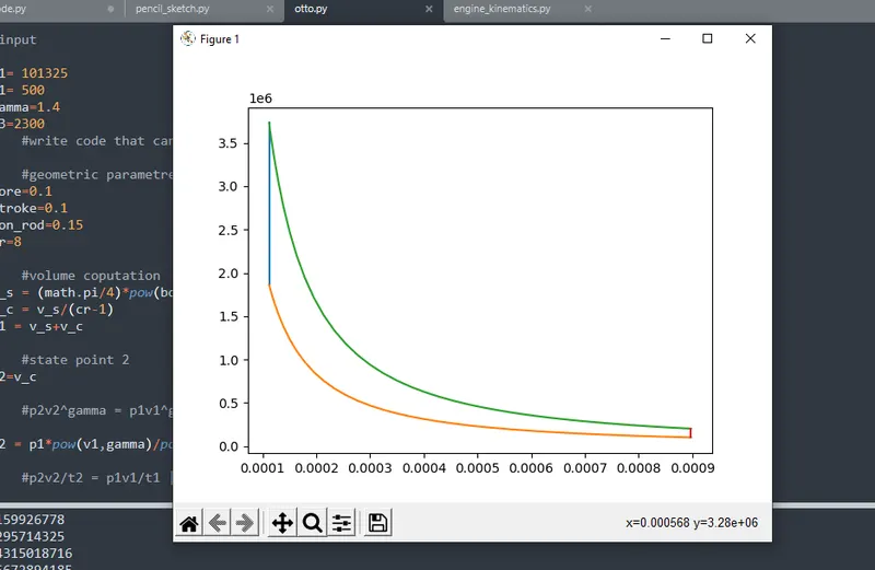
plt.plot([v2,v3],[p2,p3])
plt.plot(V_compression, P_compression)
plt.plot(V_expansion, P_expansion)
plt.plot([v4,v1],[p4,p1])
plt.show()
Explanation:
- Import import matplotlib.pyplot as plt
- Define the engine kinematics of bore,stroke,con_rod,cr,start_crank,end_crank
- Here volume parameters are taken as V_s = math.pi*(1/4)*pow(bore,2)*stroke
V_c = V_s/(cr-1) - The formula for start crank and end crank are taken as sc=math.radians(start_crank)
ec=math.radians(end_crank) - Now take the num_values = 50 and in for loop solve the equation into 3 terms as
term1 = 0.5*(cr-1)
term2 = R+1-math.cos(theta)
term3 =pow(R,2)-pow(math.sin(theta),2)
term3=pow(term3,0.5)
- Now solve them as V.append((1 +term1*(term2-term3))*V_c)
- Now solve the "V compression" AND "V expansion" as V_compression=engine_kinematics(bore,stroke,con_rod,cr,180,0) and
- P_expansion.append(constant/pow(v,gamma))
- At state point 4 solve p4 = p3*pow(v3,gamma)/pow(v4,gamma)
- After calculating varous state points we plot them in graphical form
- A function is created to calculate the valume trace using volume trace formula
- Now all the data is plotted and get desired result.