Structural Modelling using Etabs 2018

Aim: To frame the structure for the given architectural drawing for G+7 residential building and check for the satisfying design as per the code.

Introduction: From the given architectural drawing place the column and provide the frame and shear wall where required and run analysis and do the necessary check such as modal response spectrum analysis and analysis result of the etabs model for inter storey drift requirements, vertical and planar irregularities, etc.

Procedure:

• From the given architectural drawing possible framing structure to be planned before creating the model in Etabs. The fig A shows the plan of the strucutral element which will be used for creating, analysing and redesigning.

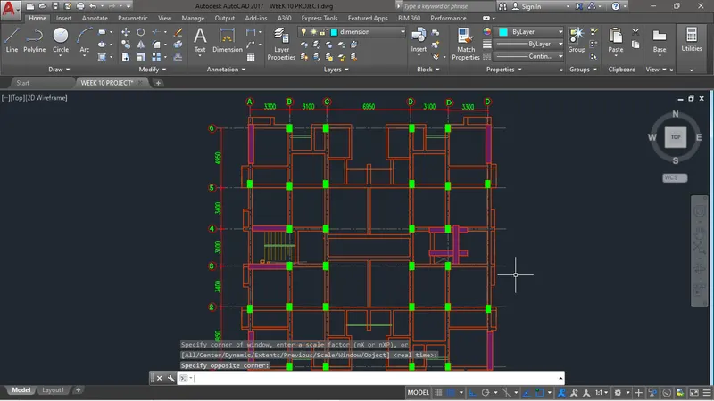
Fig A: Structural predesign concept of the given architectural plan

• Now open Etabs and create the structure as per the Planned fig A. The following fig shows the process of creating the strucuture by creating the bays, stores, defining sections and assigning them.

Fig B: Open Etabs.

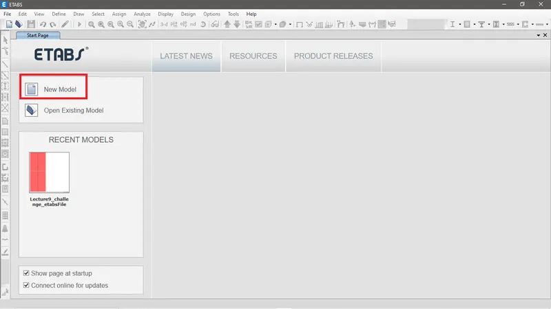
Fig C: Click on New Model

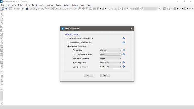
Fig D: Define the standard code required to design respective to the country.

Grid creation

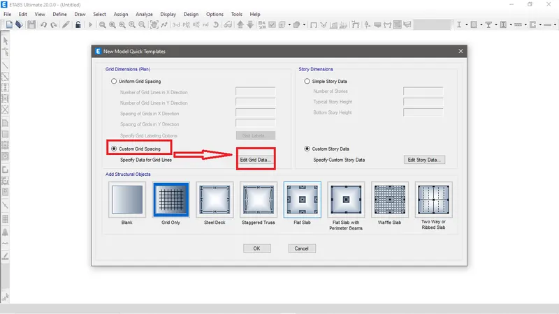
Fig E: Select grid spacing and click in Edit grid data to create grid for the strucutre.

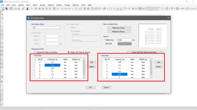
Fig F: Now specify grid in X and Y data and respective distance and click on Ok.

Storey creation

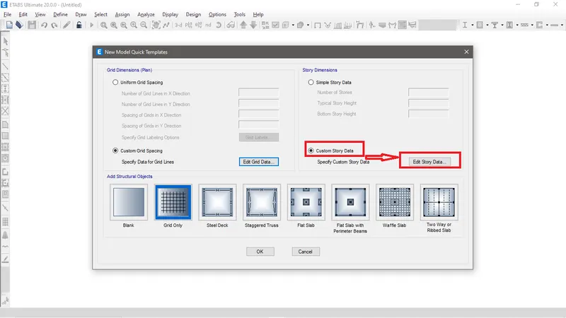
Fig G: Now select custon story data and click on edit story data to create story

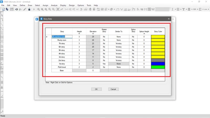
Fig H: Now add and edit story as required and click on Ok.

XYZ grids created as per requirement

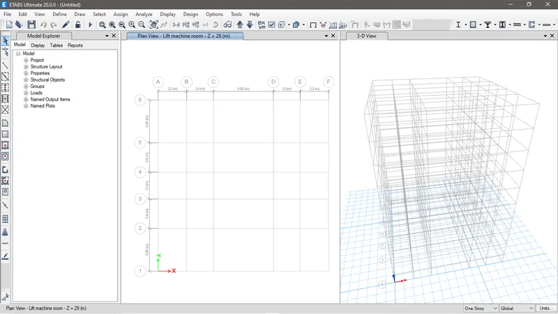
Fig I: Grid created for building strucuture.

Material defining

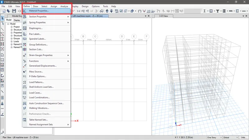
Fig J: Go to Define tab > click on Material properties

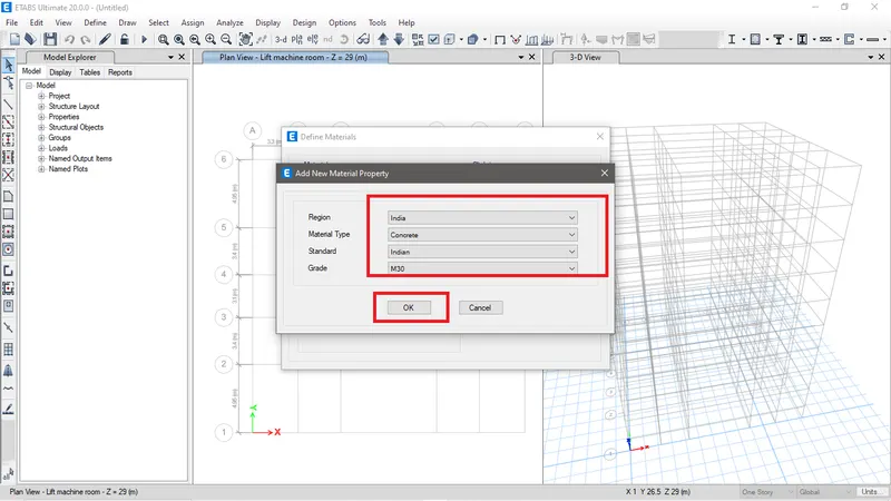
Fig K: To define concrete material select concrete in Material type and difne it grade and standard and click Ok.

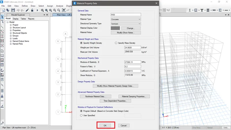
Fig L: Now click on Ok again as we dont have to edit anything as it is defined as default as per the standard code.

To define still the process is same only thing is the material type and standard code will be choosen as Rebar grade as required.

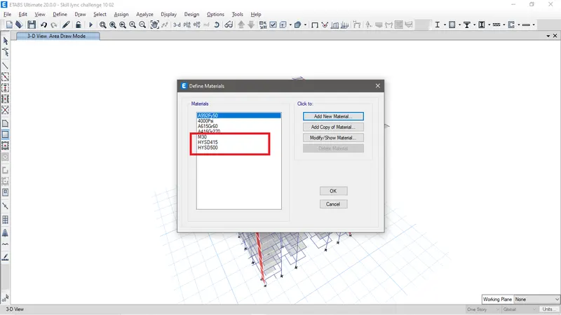
Fig M: Material properties of concrete and reinforcement is defined.

Section defining.

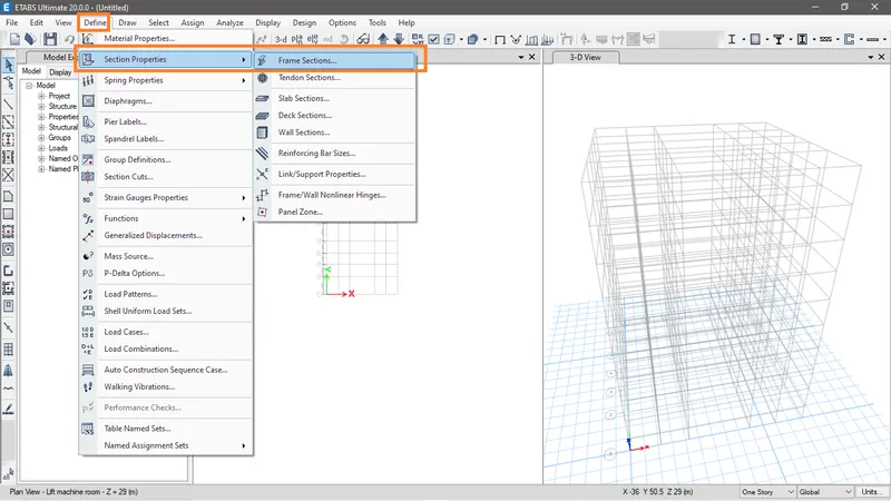
Fig N: Go to Define tab > Section Properties > Frame sections

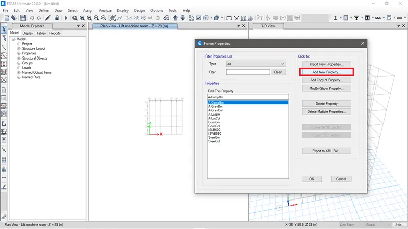
Fig O: Add new property

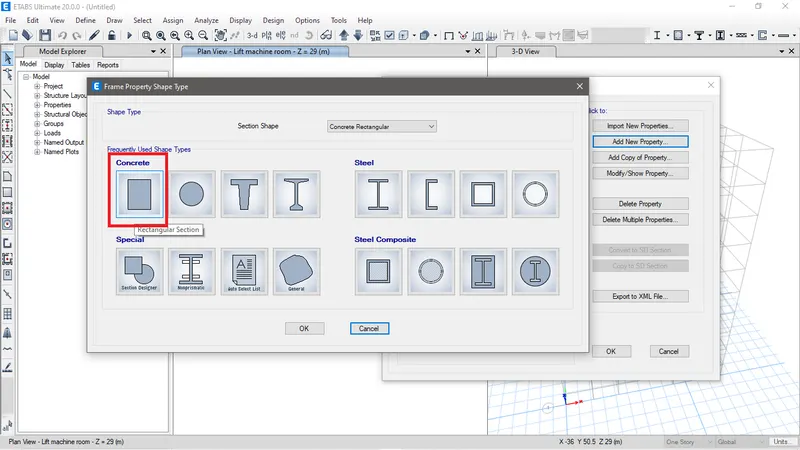
Fig P: Choose concrete shape as required.

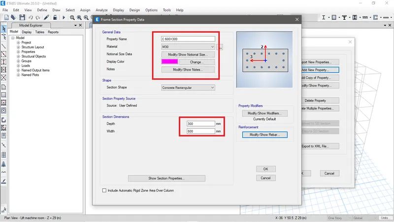
Fig Q: Now define property of sections as required and then click on Modify/show rebar to define reinforcement of the section.

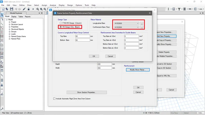
Fig R: Define the reinforcement property for the section.

Similarly many other frame sections are created in this process.

Define wall sections

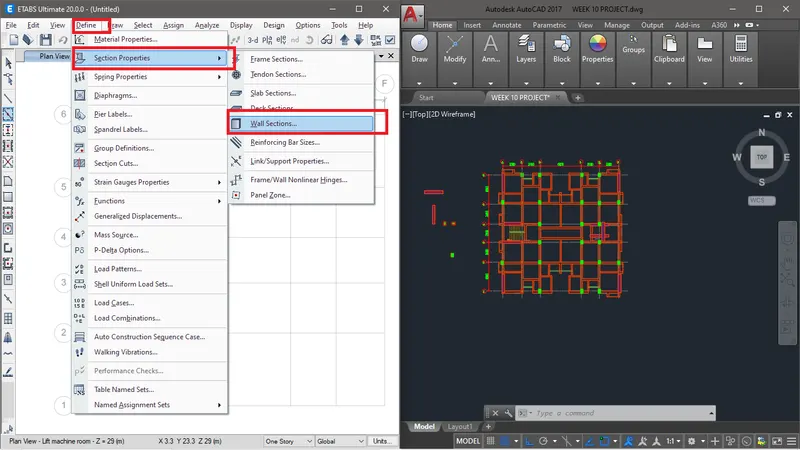
Fig S: To define wall sections go to Define tab > Section properties> Wall sections

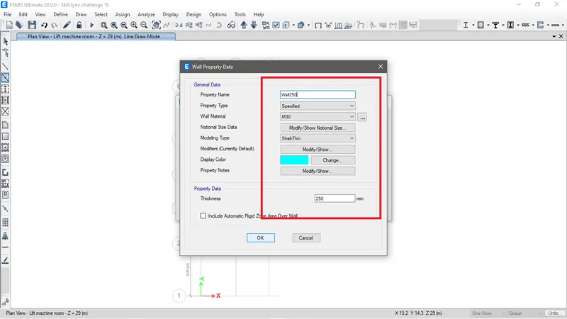
Fig T: Click on add new wall and define the property of the wall as required.

Define slab sections

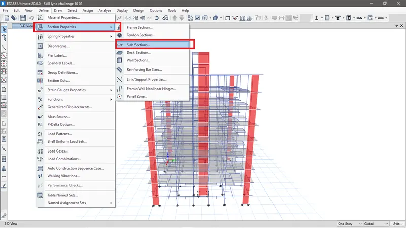
Fig U: Go to define tab > Section properties > Slab sections.

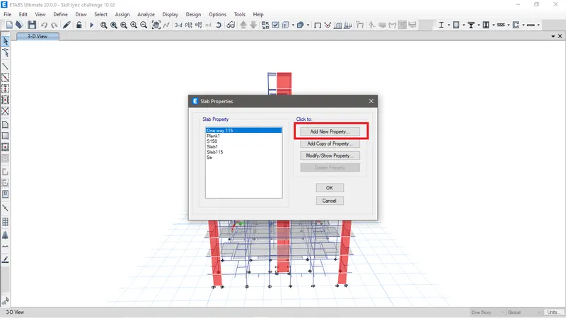
Fig V: Click on add new properety

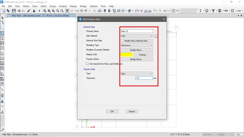
Fig W: Now define the property of the slab and then click on Ok.

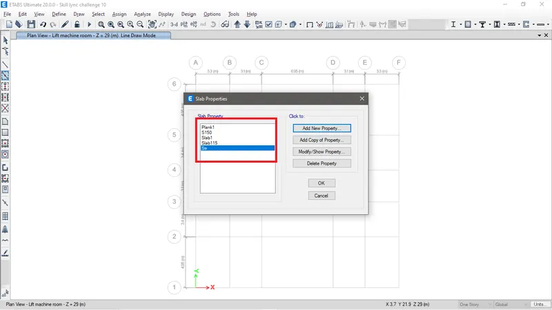
Fig X: Similarly slab of different properties are created.

Assign section to the structure.

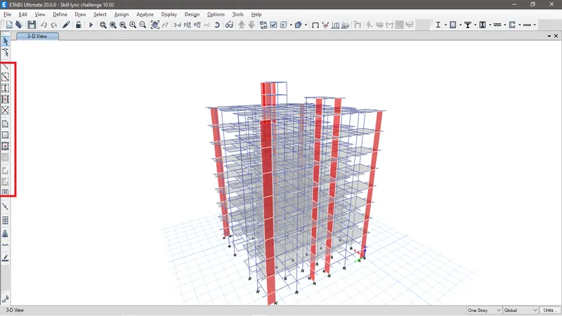
Fig Y: With the help of the draw tools sections such as column, beam, slab and shear wall to the structure are now assisgned.

Assign Fixed restrain to the base

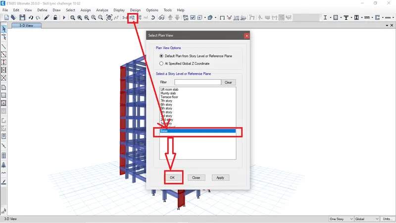
Fig Z: Go to Plan > Select base and click on Ok.

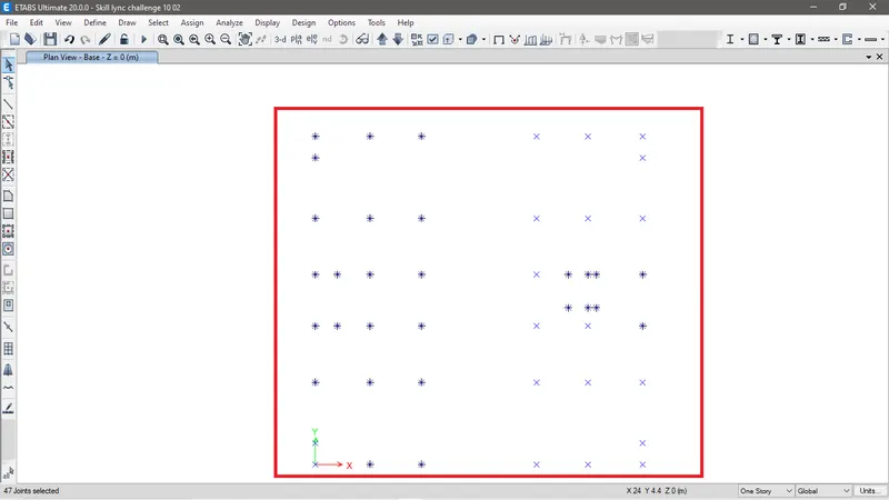
Fig AA: Now select all the joints to assign restraints.

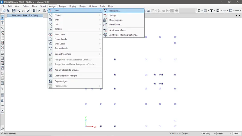
Fig AB: Now go to Assign>Joint> Restraints.

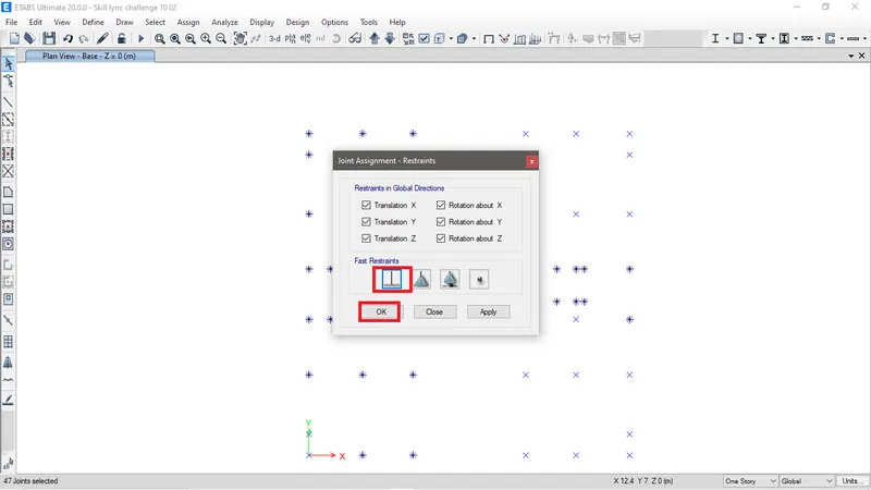
Fig AC: Now select Fixed restraints and click on OK.

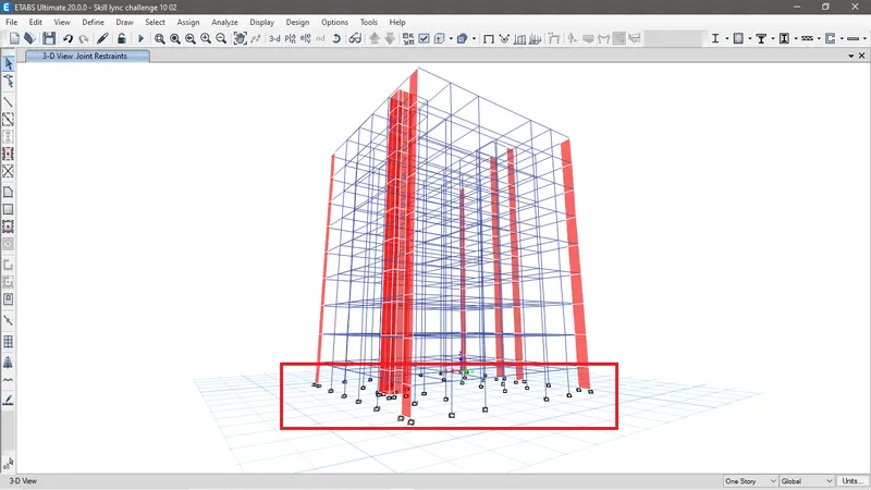
Fig AD: Fixed restraint are now assigned to the joints at base.

To define loads

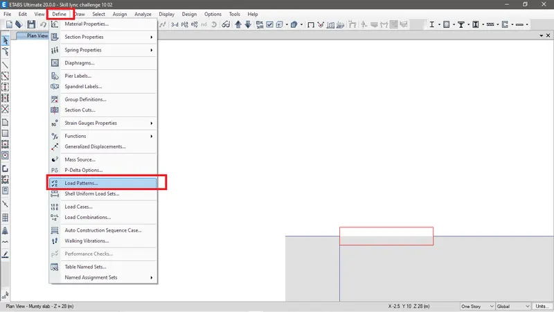
Fig AE: Go to Define tab> Load patterns.

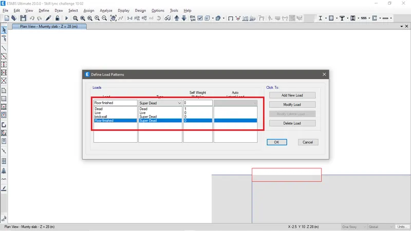
Fig AF: Add new load pattern and the click on Ok to finish.

To assign load to the structures.

Assigining brickwall load on beam. To define the load of the brickwall on beam we need to analyse and find the value of the load of the brick wall on that respective beam. In this structure the brick wall is AAC, hence the density of the AAC block 6KN/m3 and thicksness of the wall is 200mm. So the brick wall load for the following beam are calculated as below:

For the beam 300X600 mm the wall height would be = 3m - 0.6m= 2.4m

So brickwall load would be calculated as = Density of the brickwall* Height of the brick wall * Width of the brick wall = 6*2.4*0.2= 2.88 KN/m

Now considering 12mm interior finishes and 18 mm exterior plastering on brick wall, the load would be = Density of the plaster* Height of the plaster* thickness of the plaster= 20*2.4*(0.018+0.012)= 1.4KN/m

Adding both load for brickwall we get 2.88+1.4= 4.28Kn/m.

Similarly For the beam 300X450 mm the wall height would be = 3m - 0.45m= 2.55m

So brickwall load would be calculated as = Density of the brickwall* Height of the brick wall * Width of the brick wall = 6*2.55*0.2= 3.06 KN/m

Now considering 12mm interior finishes and 18 mm exterior plastering on brick wall, the load would be = Density of the plaster* Height of the plaster* thickness of the plaster= 20*2.4*(0.018+0.012)= 1.4KN/m

Adding both load for brickwall we get 3.06+1.4= 4.46Kn/m.

Moving ahead to assign load to the frame.

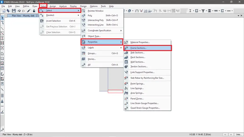
Fig AG: First select sections to assign the load. To do that go to Selec tab> Select> Properties> Frame sections

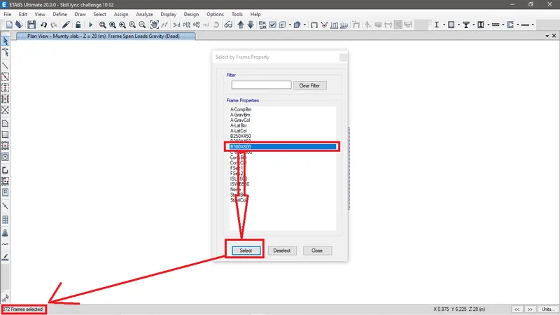
Fig AH: Now select sections required to be selected and click on select. We can see numbers of section selected in the structure.

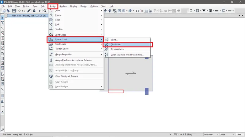
Fig AI: Now, go to Assign> Frame Loads> Distributed.

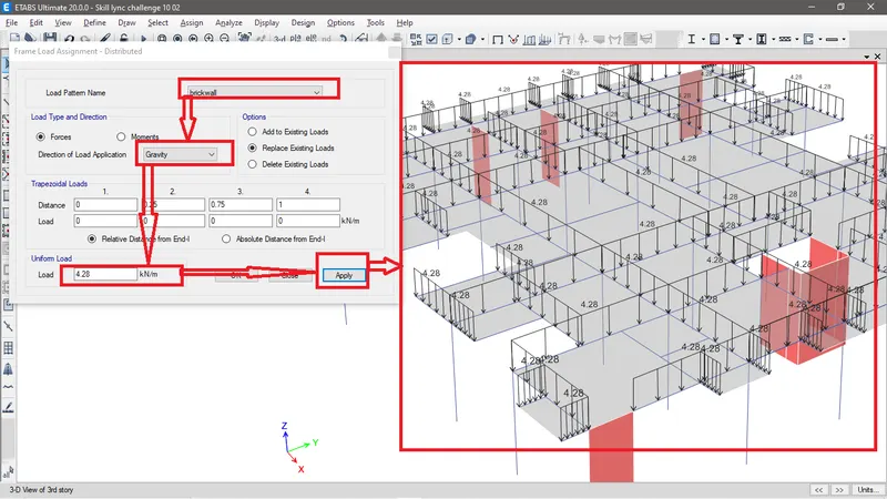
Fig AJ: Now define the load pattern name and provide the load and click on apply. We can see the load has been assigned to the selected sections. Similarly the loads are assigned to remaining frame sections.

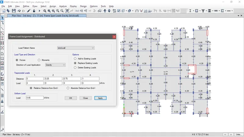
Fig AK: Loads assigned to remaining sections.

Assigning Live load and Floor finished load to slab section.

Following the codal provision of IS 875 part 2 for live load.

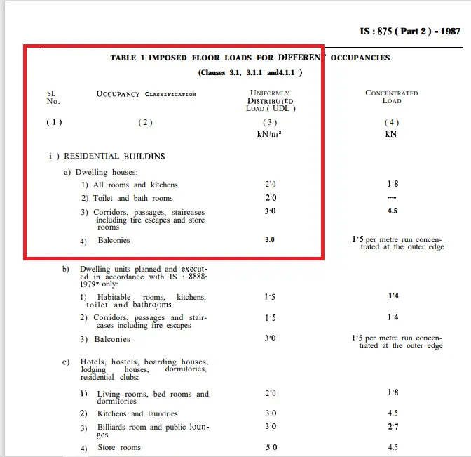
Fig AL: Taking value from Table 1 of IS875 Part 2 for live load on slabs

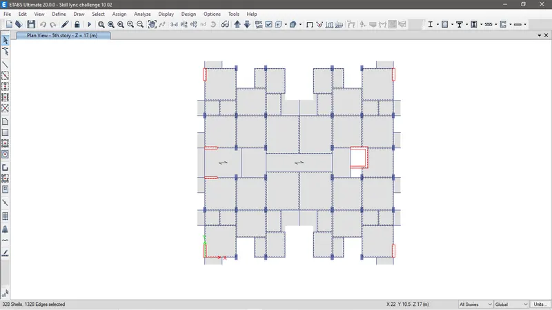
Fig AM: Select all rooms, Kitchen, Toilets

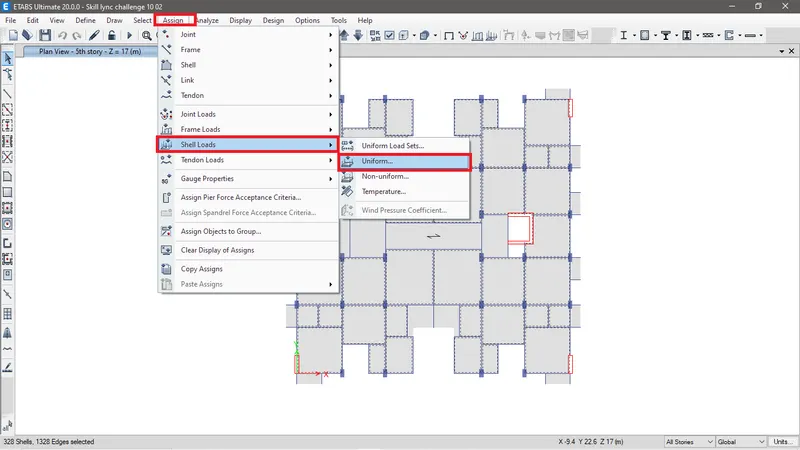
Fig AN: Go to assign tab> Shell loads > Uniform

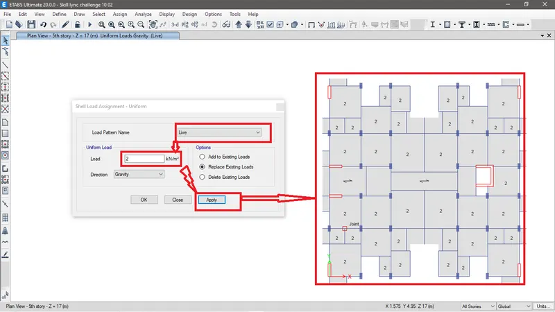
Fig AO: Now select load pattern name as live to assign live load and provide the value as per the code and then click on apply. We can see that all the selected slabs are now assigned with respective live load. Similarly select the slab for different live load and assign it.

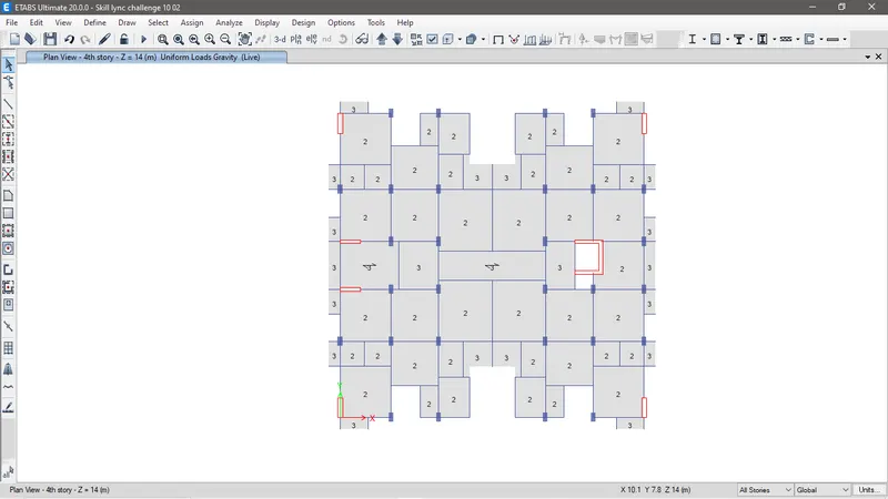
Fig AP: Now all the slabs are assigned with live load respected to their load as per IS 875 part 2 Table 01

Similarly floor finished loads are assigned by just choosing load pattern name as floor finished load and providing respective load to the respective slab.

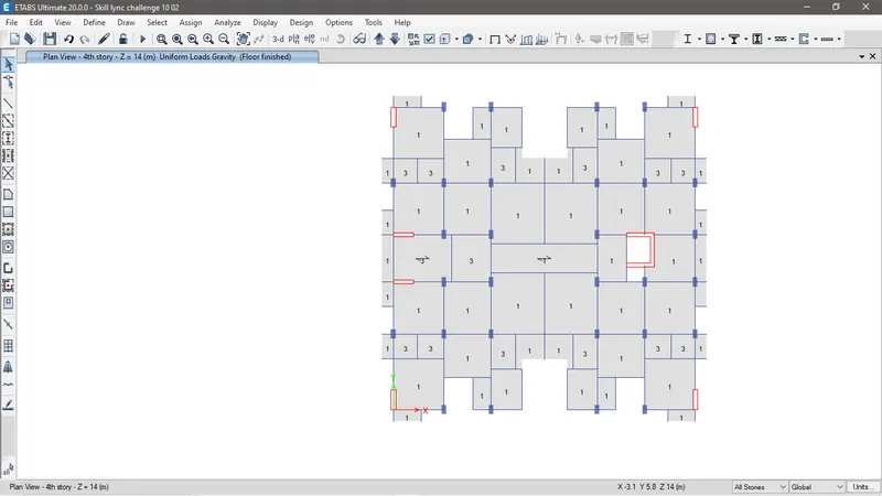
Fig AQ: Floor finished load assigned to the given slab.

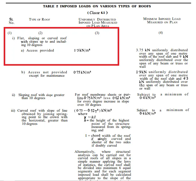
Fig AR: But as per IS 875 part 2 Live load for flat room is 1.5KN/m2.

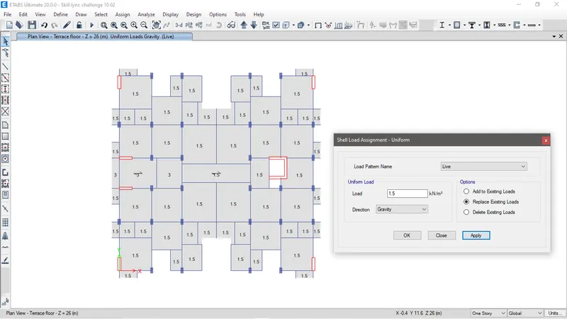
Fig AS: Live load of 1.5KN/m2 is assigned to the flat roof as per IS code.

On Mumty roof slab Water tank of 20000L will be provided so the super dead load of the Mumty slab would be calculated as the following.

Weight of the water is 20000Kg.

20000L = 20Cum.

since the length of the staircase is 6m and 3.1m. The area of the Mumty slab would be 18m2. So the depth of the water tank would be

Volume of the water tank / Area of the mumty slab= 20m3/18m2= 1.1m

Hence super dead load for the mumty slab would be

Weight of the water Kn/m3* height of the water tank= 9.81Kn/m3*1.1m=11Kn/m2.

Now to apply super dead load on Lift machine room floor. The load should be applied as per the manufacturer requirement. IS 875 Note 9 page no 12 states it such a way.

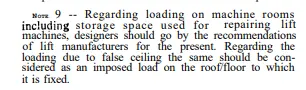
Fig AT: IS 875 Note 9: statement of lift machine load on floors.

Live load reduction factor

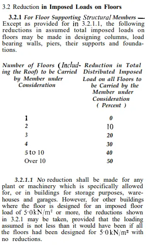
Fig AU: IS 875 clause 3.2 states about Live load reduction factor.

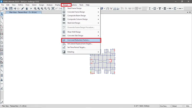
Fig AV: To define live load reduction factor in Etabs. Go to Design tab > Live load reduction factors...

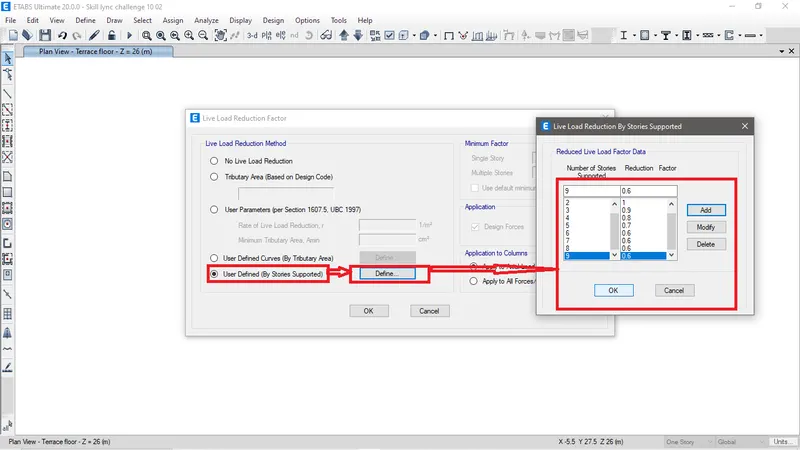Fig AW: Now select user defined (By stories supported) > click on Define > later define reduction factor for each stories by adding and click OK when finished.

Defining seismic load.

Points to note to apply seismic load. We must know Seismic zone, Soil type, time period and reduction factor. The code book to follow for Seismic load is IS1893-2016.

The siesmic zone is 5, soil type assume as II.

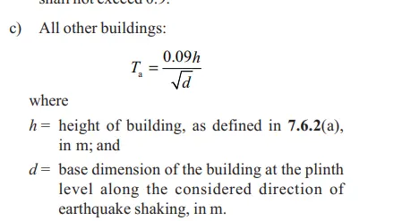
Fig AX: Time period formula for the strucuture as per IS 1893 - 2016

Here the h= 30m and the Length of the building on both the directions are 20 m

So Ta= 0.09*30/Sqrt(20)= 0.60 sec.

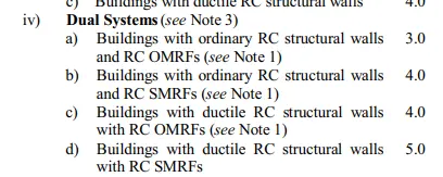
Fig AY: From IS 1893 - 2016 considering the structure to be dual system and is a building with ductile RC structural walls with RC SMRFs. Hence the Response reduction factor for the building R is 5.0

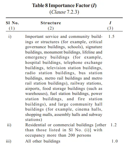
Fig AZ: From IS 1893-2016 Table 8 the importance factor for the building will be 1.0 as this building fall under category iii.

Now with the all above values the seismic load will be define with respect ot X and Y direction both negative and positive form.

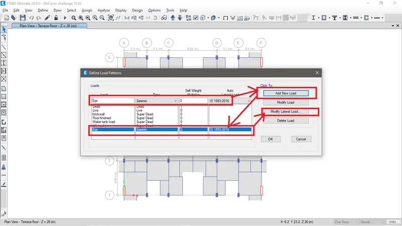
Fig AZ: To define seismic load go to Define tab > Load pattern > Define and and the load and then click on modify lateral load to define its properties.

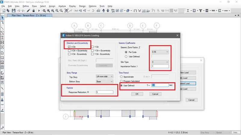
Fig BA: Now the Properties are defined for Eqx. Similarly the Properties for rest of the seismic load with respective to the direction will be defined.

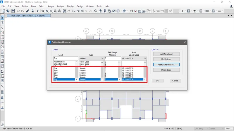
Fig BC: All the seismic load is being defined.

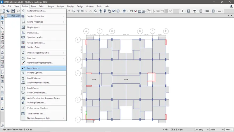
Fig BD: To analyse seismic load mass source of the building has to be defined. Go to Define tab > Mass source

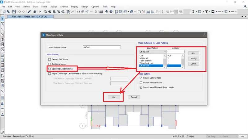
Fig BE: Now check specified load patterns and define all the load patterns and click on OK.

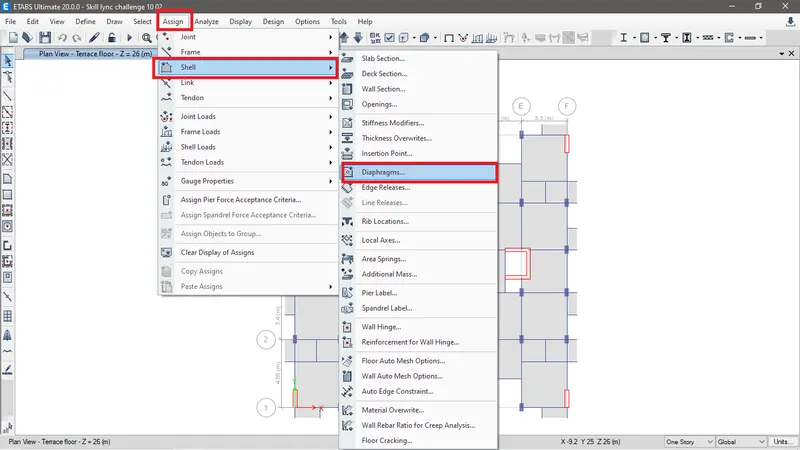
Fig BF: To assign diaphragms first select all the slabs section and then go to Assign tab > Shell > Diaphragms.

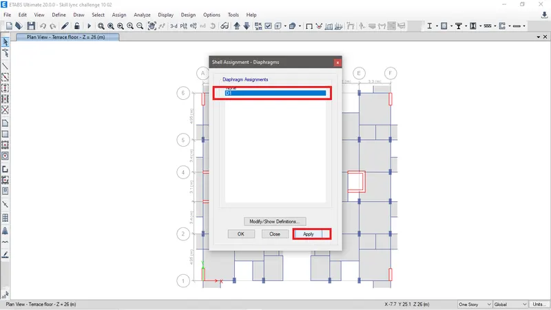
Fig BG: Select D1 and click on apply.

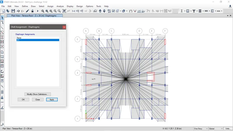
Fig BH: Diagphram is now applied.

Defining load combination

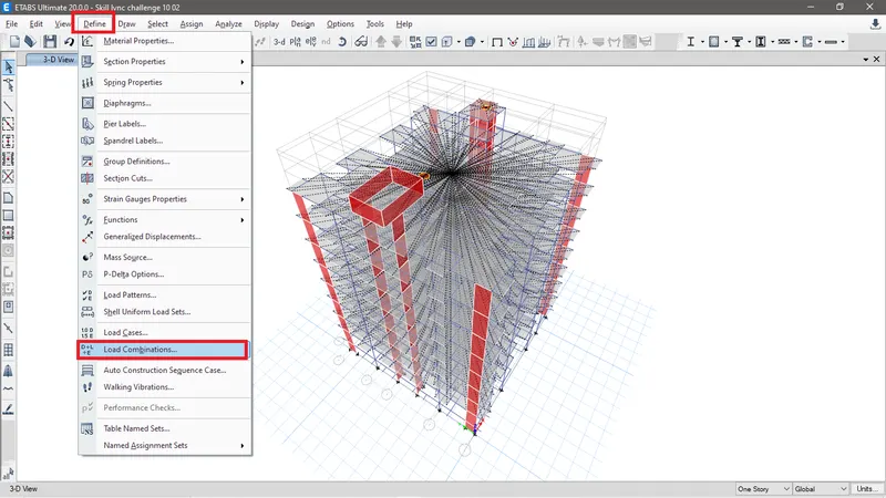
Fig BI: Go to Define tab> Load combinations.

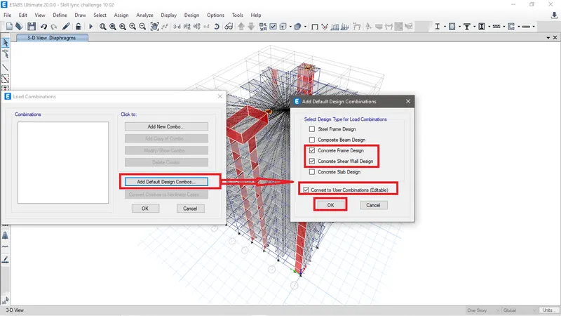
Fig BJ: Click on Add default Design combos and check Concrete frame design, Concrete shear wall design and Convert to User Combinations (Editable) and then click OK.

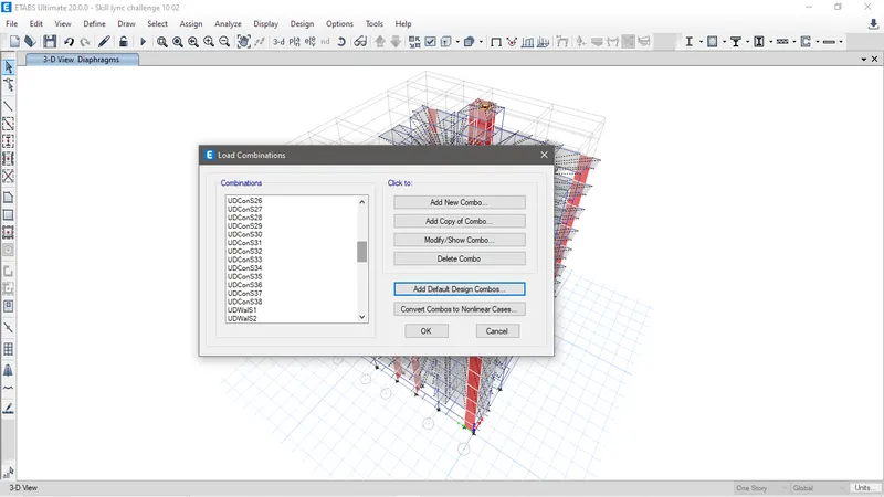
Fig BK: All load combinations are now defined.

Check the load cases and edit the modal case if required.

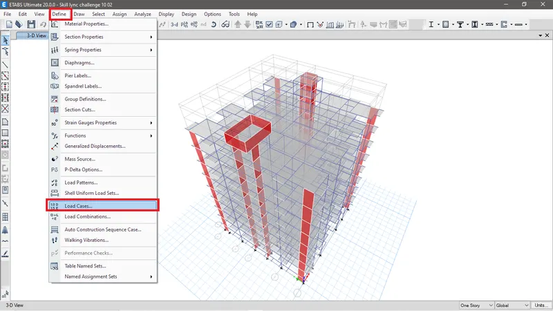
Fig BL: To check the load cases go to Define tab > Load cases.

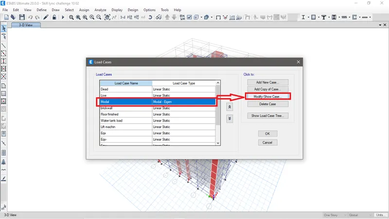
Fig BM: Select the Modal case and click on modify/show case.

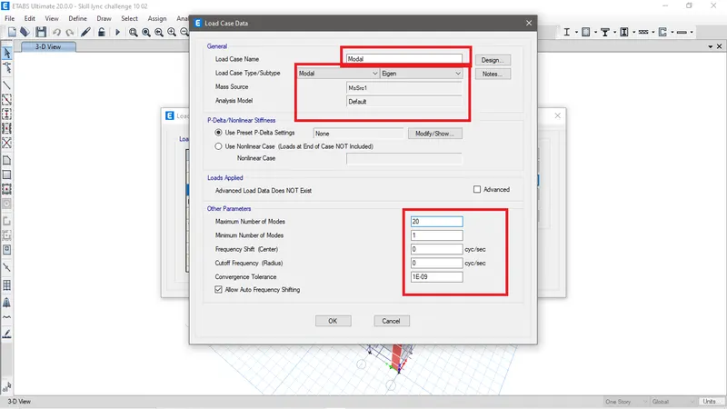
Fig BN: Define the modal case data as required.

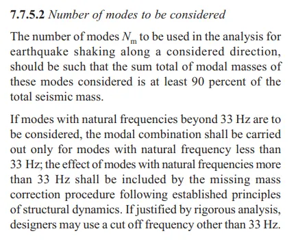
Fig BO: Number of modes in modal cases to be considered as per IS 1893-2016 Clause 7.7.5.2.

To set load cases to run.

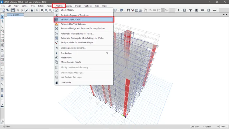
Fig BP: To set load cases to run go to analyze tab > Set load cases to run.

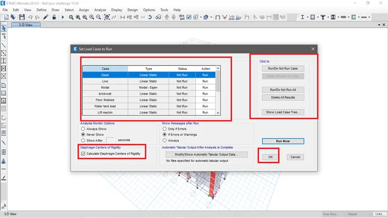
Fig BQ: Now select load cases to run or not run the case and check the calculate diagphragm centre of rigidity and then click OK.

To check the model for any error or clashes in model.

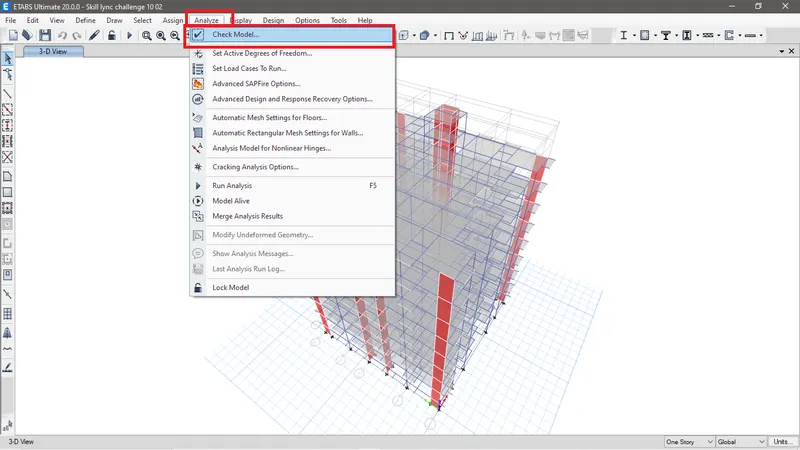
Fig BR: To check the model go to Analyze tab> Click on Check model

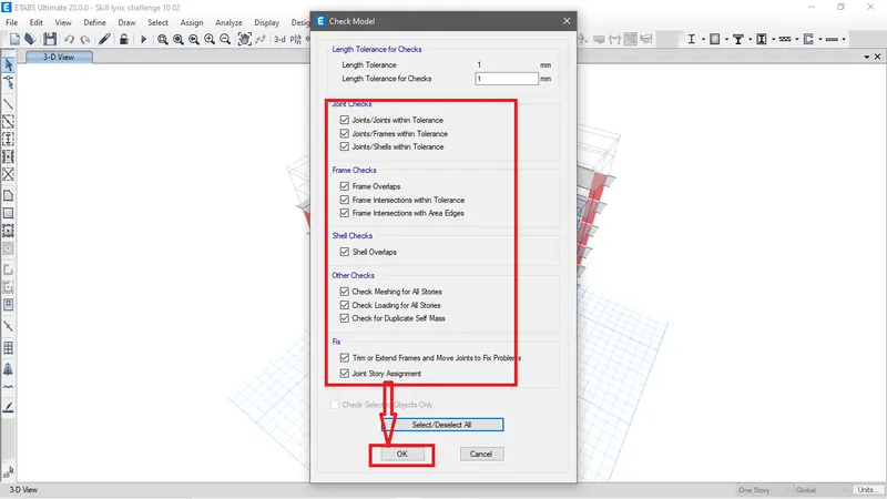
Fig BS: Check all the required boxes to check and then click OK.

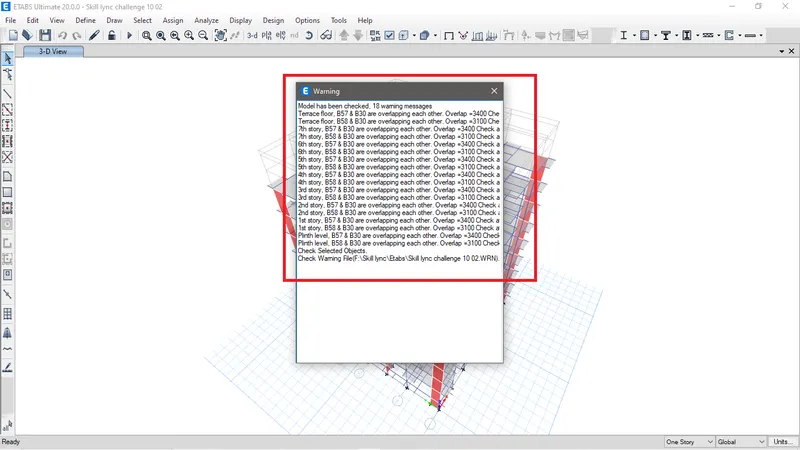
Fig BT: We receive warning if it is available after some runs. With this warning location the error is identified and corrected.

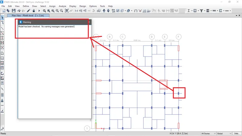
Fig BU: The error was identified as shown in the figure. After correcting the error, when we recheck the model we receive no warning note.

To define response spectrum function.

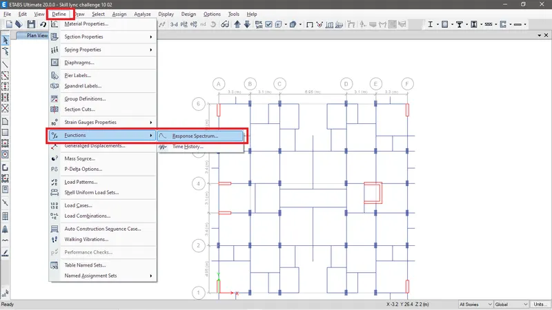
Fig BV: Go to Define tab > Functions > Response spectrum.

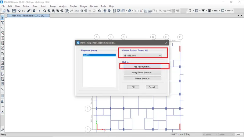
Fig BW: Select the respective code and then click on add new functions.

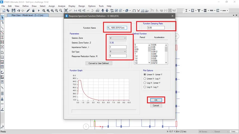
Fig BX: Do necessary changes and click on Ok.

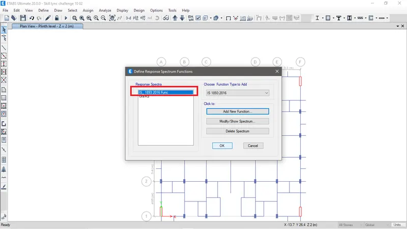
Fig BY: Required response spectrum function is added.

Add response spectrum load cases.

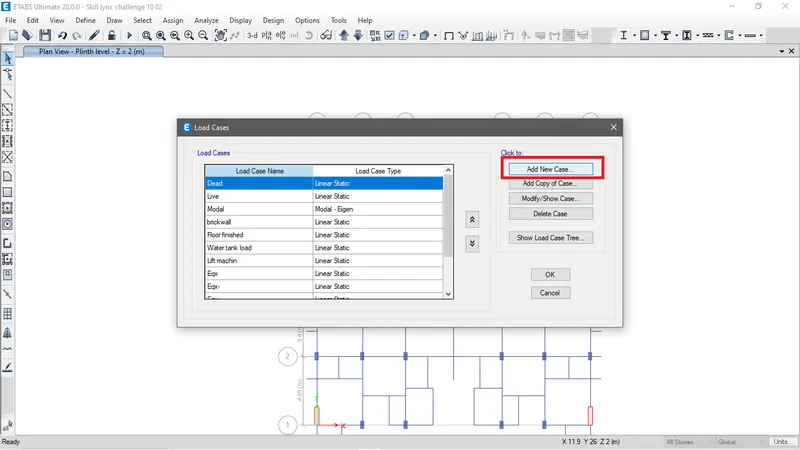
Fig BZ: Go to load cases and click on add new case.

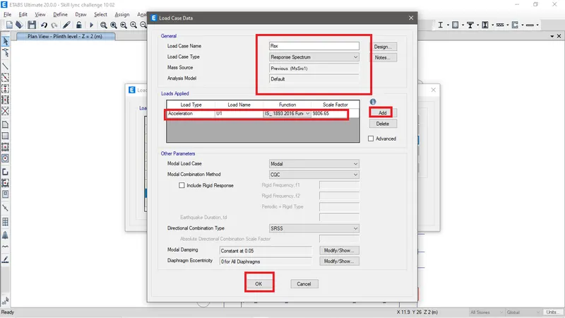
Fig CA: Define the name of this load and click on Add and choose Load name as U1, Select function as defined and Scale let it remain the same. This scale factor will be altered after running the analysis and seeing that the base shear Vb reaction of Eqx and Rsx is similar or not. If the base shear reaction is not same then the value will be corrected by recalculating as per IS 1893 - 2016 clause 7.7.3.

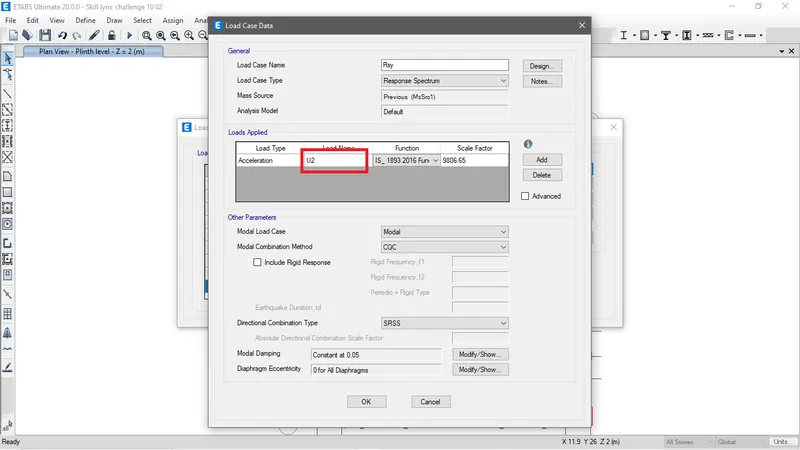
Fig CB: Similarly for Response spectrum load in Y direction will be defined the name of this load and click on Add and choose Load name as U2, Select function as defined and Scale let it remain the same.

c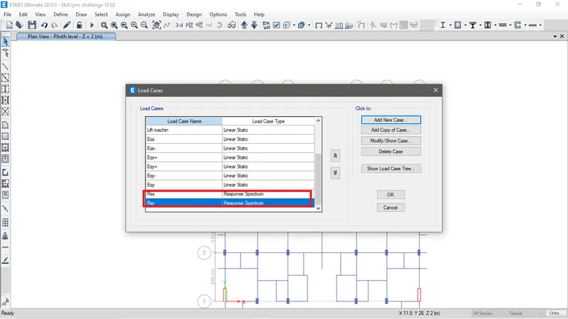

Fig CC: We can see that response spectrum load case for both X and Y directions are added.

(Note: If there is any changes done in load cases do delete all the load combinations and readd the load combination. So that the loadcombinations are updated.)

Run analysis to understand the base shaear reactions of lateral load X and y direction and Response spectrum load in X and Y direction.

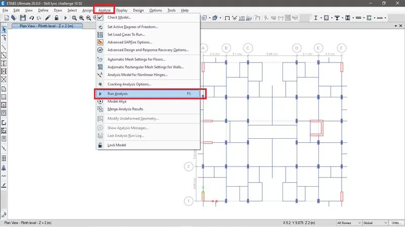
Fig CD: Go to Analyze tab > Click on Run analysis.

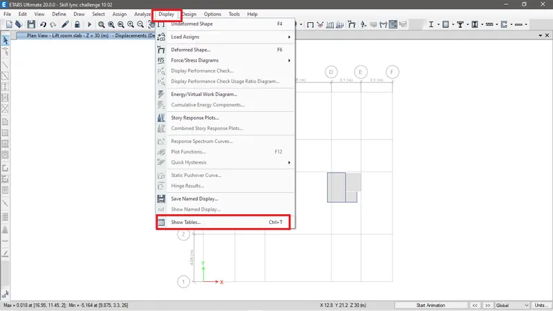
Fig CE: Now go to Define tab > Show tables

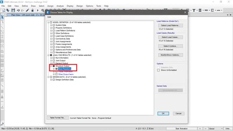
Fig CF: Select Base reactions and click on Ok.

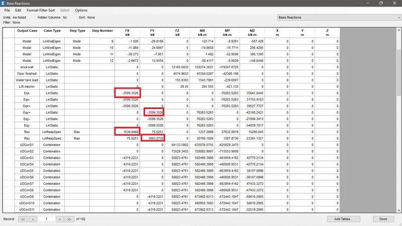
Fig CG: We can see in the fig that the result of the response spectrum both in X and Y direction that is Rsx and Rsy is less than the Eqx and Eqy.

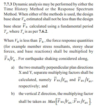
Fig CH: Hence as per IS 1893: 2016 clause 7.7.3 if the response spectrum base shear is less then the fundamental response then the scale factor of the response spectrum load case should be corrected by multiplying with value Vb'/Vb.

From Fig CA and CB the scale factor for Rsx And Rsy is 9806.65

So the corrected value of the scale factor for Rsx is (3599.35/1539.85)*9806.65= 22947.56

So the corrected value of the scale factor for Rsy is (3599.35/1663.27)*9806.65= 21221.79

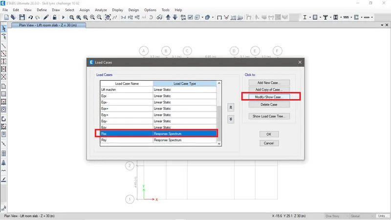
Fig CI: Now go to load case and select the Rsx and click on Modify/show case.

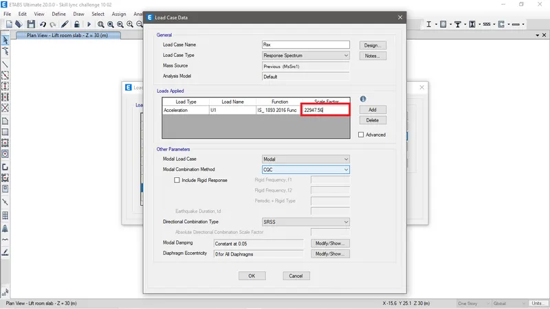
Fig CJ: Now use the corrected scaled factor value in Rsx load case and click OK. Similarly do the same to Rsy.

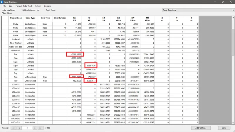
Fig CK: Re run the analyze and we can see the base shear reaction for Eqx, Eqy, Rsx and Rsy is similar.

Now since we have modelled and corrected the scale factor for response spectrum force and defined all the load cases. Now let's save the file in 3 different form. One file where the only gravity load on the structure will be anlaysed, second lateral load will be analysed and third response spectrum will be analysed.

Note: In File anlayzing only gravity load will contain load cases only gravity load and the moment of intertia for Beam and column will be 1

In file analyzing lateral load will contain load cases gravity, Eqx, Eqy and their positive and negative load and having moment of inertia for column 0.7 and beam 0.3.

In file analyzing Response spectrum force will contain load cases gravity, Eqx, Eqy Rsx and Rsy and having moment of inertia for column 0.7 and beam 0.3.

Structural ananlysing gravity load only.

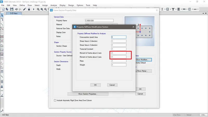
Fig CL: Moment of inertial about 2 and 3 axis are defined 1.

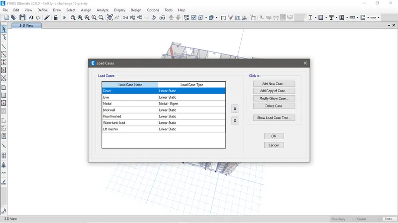
Fig CM: Only gravity load cases are defined.

Now re add the combination of the load and check the model and run analysis and do the necessary checks.

Check the uplift of the structure.

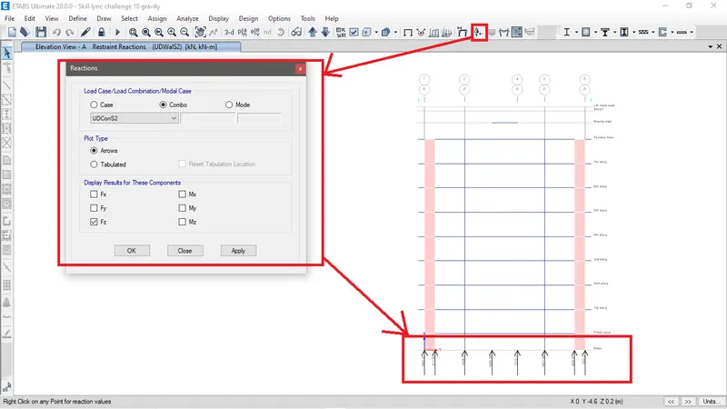
Fig CN: Go to support reaction and select combo and check force and Z direction and click on apply. No uplift to be seen in any columns and hence good to go.

check the axial load ratio on column and shear wall.

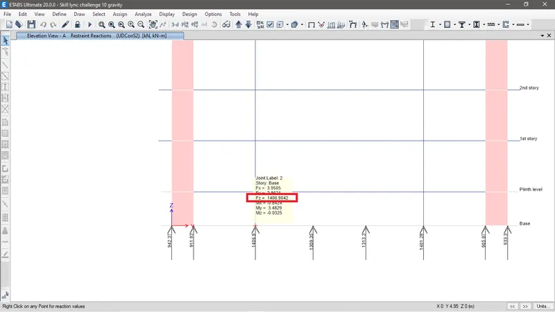
Fig CO: It is to be noticed that the force on column is 1406KN

From calculating

((1406*1000)/(300*600))/30= 0.26.

As per IS 13290 the vertical support should take max 40% of Fck and the load in this column is within the limit. Hence it is permissible.

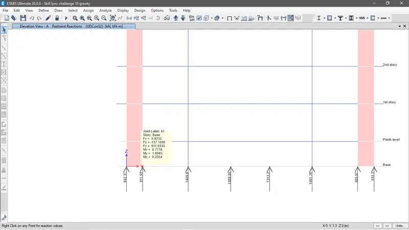
Fig CO: It is to be noticed that the force on shear wall is 911KN

From calculating

((911*1000)/(300*600))/30= 0.17.

As per IS 13290 the vertical support should take max 28% of Fck and the load in this shear wall is within the limit. Hence it is permissible.

Structural ananlysing Lateral load.

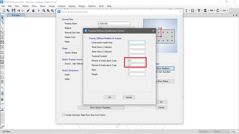
Fig CP: Moment of inertial is 0.7 for column

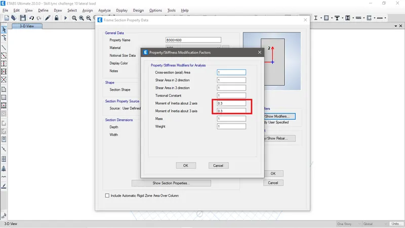
Fig CQ: Moment of inertial is 0.3 for beam

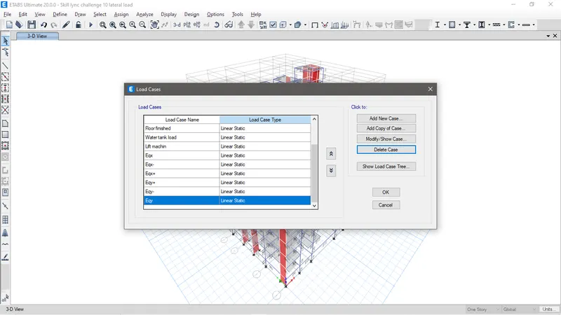
Fig CR: These are the load cases defined for anlayzing lateral load forces on structure.

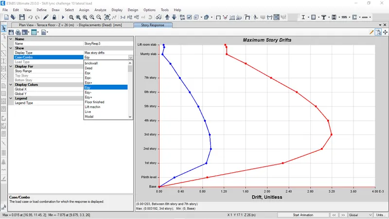
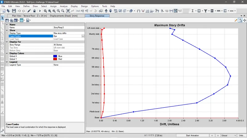
Fig CS: After run analsis the Max story drift for bothe Eqx and Eqy is with 0.4% hence it is permissible.

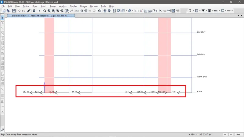
Fig CT: This are the base shear reaction of the wall at Eqx direction.

By adding total base shear force of the shear wall and dividing it with total base shear at X direction we get

(1171*2)/3500=0.67

Required minimum 0.75 to 0.80 of the total base shear force gone to shear wall. Here this may be allow but increasing the number of shear wall or the size may satisfy the result.

Now checking base shear reaction of wall in Y direction.

The total base shear of the walls along Y direction are 1368Kn.

2303/3500= 0.66

Required minimum 0.75 to 0.80 of the total base shear force gone to shear wall. Here this may be allow but increasing the number of shear wall or the size may satisfy the result.

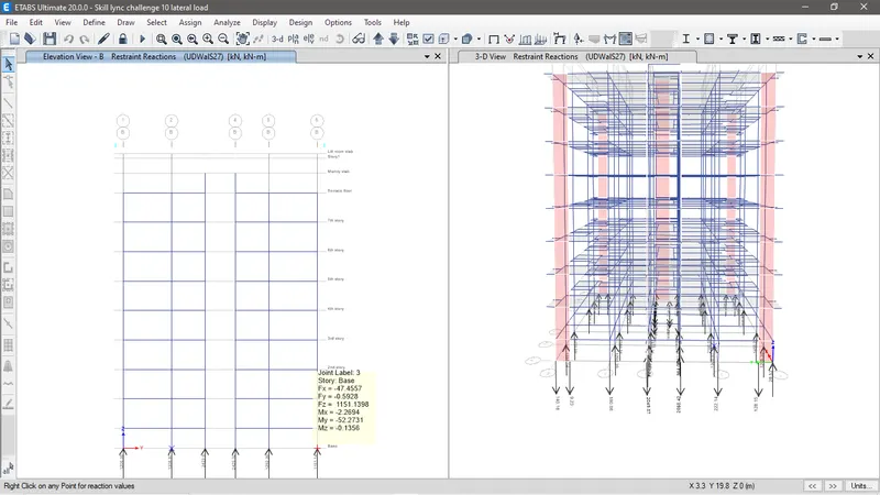
Fig CU: While checking base force reaction on Z direction by applying 0.9 load combo on structure we see that some of the column are undergoing tensional force and some of the column is having load more than the 40% of the fck. This performance of the structure will not be permissible. Hence we need to provide better section of the vertical support for better stability of the strucuture.

Structural analysing Response spectrum.

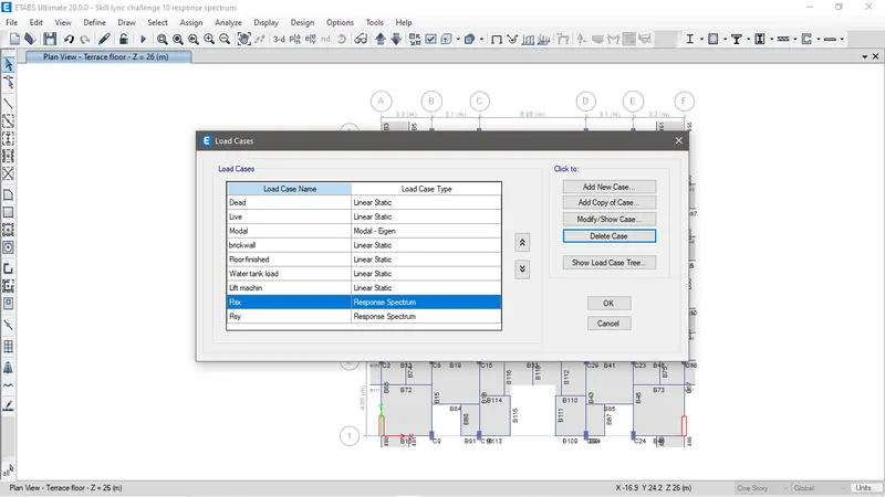
Fig CV: Load cases to be considered for response spectrum analysis is Gravity load and Response spectrum load.

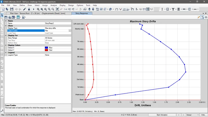
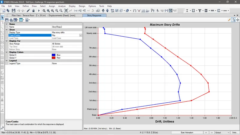
Fig CW: Story drift in response spectrum analysis is satisfying as it is below 0.4% both in X and Y direction.

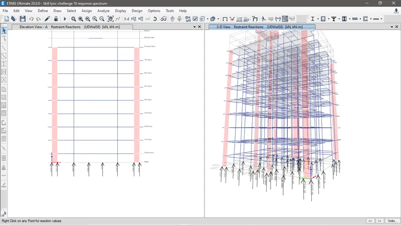
Fig CX: Force reaction on column and shear wall looks good and satisfying.

The base shear is distributed only 66% on shear wall. The shear wall to be altered for better shear distribution.

Conclusion

After different load analysis it is found out that the base shear force is quitly well distributed on shear wall.

The gravity load analysis and response spectrum analysis do show some good results in distributing the load on vertical support and shear wall.