Structural dynamics
1.0
AIM: To differentiate static and dynamic analysis.
INTRODUCITON: In this week basics of structural dynamics analysis is covered with explaination the following topics.
- Differentiation between static and dynamic analysis
- Force displacement graph for linear elastic as well as for linear inelastic system
- Components in equation of motion such as mass, stiffness and damping components
- Concept of period of vibration, frequency of vibration
- Response spectrum and graph related it.
Difference between static and dynamic analysis:
- A static analysis can only be performed if the system being simulated does not depend on time, and if the loads being applied are constant. In a dynamic analysis, the system itself, the load application, or both might change with time.
- In a dynamic analysis, the inertial loads developed by the system due to acceleration are taken into account. Static analysis don’t consider inertia.
- Mathematically, the difference between static and dynamic analysis is that in a static analysis, only the stiffness matrix of the FEA model is solved. In a dynamic analysis, in addition to the stiffness matrix, the mass matrix (and damping matrix, if not zero) is solved as well. That is one of the reasons why dynamic analyses require more computational time than static analyses, for the same structure.
- For a dynamic analysis, the loads can be in either the time domain or in the frequency domain.

RESULT: I understood difference between static and dynamic analysis.
2.0
AIM: To understand relevant graphs of following
- Elastic behavior
- Inelastic behavior
- Plastic behavior
- Non-linear Inelastic behavior.
INTRODUCTION: In this week basics of structural dynamics analysis is covered with explaination the following topics.
- Differentiation between static and dynamic analysis
- Force displacement graph for linear elastic as well as for linear inelastic system
- Components in equation of motion such as mass, stiffness and damping components
- Concept of period of vibration, frequency of vibration
- Response spectrum and graph related it.
1. Elastic behaviour:
Ductile materials undergo a large amount of deformation before failing. The following figure shows the stress-strain curve for a ductile specimen:
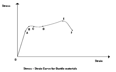
Proportional Limit: This limit is represented by point A on the graph. Up to this limit, the stress and the strain induced in the specimen are directly proportional to each other, i.e. the specimen obeys Hooke’s law. Beyond this point, the stress is not proportional to the strain.
Elastic Limit: This limit is represented by point B on the graph. Upto this limit, the material is said to be elastic. This implies that the specimen regains its original shape and dimensions after the removal of the external load. There are no residual deformations seen in the specimen, on removal of the load. After this point, the material is said to become plastic.
2. Inelastic behaviour:
This stage occurs when there is deformation produces in material without applied any force on material.
3. Plastic behaviour:
Yield Point: Contrary to what the name suggests, this is a region rather than a point. It is limited by the upper yield point ‘C’ and the lower yield point ‘D’. The stress – strain curve in this part of the graph is almost horizontal, which implies that there is an appreciable increase in strain for a negligible increase in stress. Yielding starts at ‘C’ and ends at ‘D’. After the point ‘D’, the material, due to strain hardening again starts taking load and the curve rises, as seen in the figure. The material now is said to be plastic and the deformation is of nearly permanent nature.
4. Inelastic linear deformation:
For inelastic linear deformation when we applied force on material then it will follows annother path and when we realise the force then it follows another path.
That means there are same value of defomation for different forces applied.
3.0
AIM: To explain stiffness, mass and damping components in dynamic analysis.
INTRODUCTION:
In this week basics of structural dynamics analysis is covered with explaination the following topics.
- Differentiation between static and dynamic analysis
- Force displacement graph for linear elastic as well as for linear inelastic system
- Components in equation of motion such as mass, stiffness and damping components
- Concept of period of vibration, frequency of vibration
- Response spectrum and graph related it.
Stiffness Component:
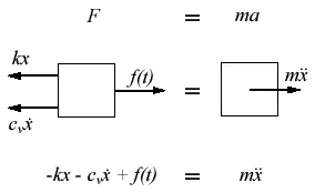
The equation of motion is, Fs+Fd+ma = P. if the external force p is applied on structure.
In this equation the Fs is the component of stiffness.
Fs = ku , where
k - stiffness coefficient which is depend on material that why introduce in the equation.
u - Displacement of structure during the earthquake.
Fs - Stiffness force required for to resist lateral force of earthquake.
Mass components:
The equation of motion is, Fs+Fd+ma = P. if the external force p is applied on structure.
According the newton's 2nd law
F = ma this the mass component in the equation of motion. and a is the acceleartion create during the lateral motion of structure.
Damping components:
When the structure is subjected to dynamic analysis then structure may vibrated. That why the damping components come in equation of motion.
Fd = cv is the damping components.
c - damping coefficent it is depends upon material that why come in equation
v - velocity with which the structure move during the lateral motion
RESULT: I understood components of equation of motion of dynamic analysis.
4.0
AIM: To explain concept of period and frequency of vibration.
INTRODUCTION: In this week basics of structural dynamics analysis is covered with explaination the following topics.
- Differentiation between static and dynamic analysis
- Force displacement graph for linear elastic as well as for linear inelastic system
- Components in equation of motion such as mass, stiffness and damping components
- Concept of period of vibration, frequency of vibration
- Response spectrum and graph related it.
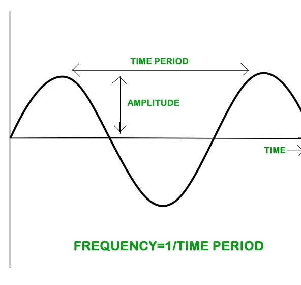
Period of vibration: Time require to complete one complete vibration cycle to structure is know the period of vibration.
Formula for period is,
T = 2π/√(k ÷ m).
Frequency of vibration:
An object's natural frequency is the frequency or rate that it vibrates naturally when disturbed. Objects can possess more than one natural frequency and we typically use harmonic oscillators as a tool for modeling the natural frequency of a particular object.
When calculating the natural frequency, we use the following formula:
f = ω ÷ 2π
We know that,
ω = √(k ÷ m)
therefore,
f = √(k ÷ m) ÷ 2π
The relation between period and frequency is as follow:
T = /f
unit of period is second s.
unit of frequency is s-1/ Hz.
RESULT: I understood concepts period and frequency of vibration.
5.0
AIM: To understand response spectrum and graph related it.
INTRODUCTION: In this week basics of structural dynamics analysis is covered with explaination the following topics.
- Differentiation between static and dynamic analysis
- Force displacement graph for linear elastic as well as for linear inelastic system
- Components in equation of motion such as mass, stiffness and damping components
- Concept of period of vibration, frequency of vibration
- Response spectrum and graph related it.
Reponse Spectrum:
Response spectrum analysis is a method to estimate the structural response to short, nondeterministic, transient dynamic events. Examples of such events are earthquakes and shocks. Since the exact time history of the load is not known, it is difficult to perform a time-dependent analysis. Due to the short length of the event, it cannot be considered as an ergodic ("stationary") process, so a random response approach is not applicable either.
A response spectrum is a function of frequency or period, showing the peak response of a simple harmonic oscillator that is subjected to a transient event. The response spectrum is a function of the natural frequency of the oscillator and of its damping. Thus, it is not a direct representation of the frequency content of the excitation (as in a Fourier transform), but rather of the effect that the signal has on a postulated system with a single degree of freedom (SDOF).
Analysis of an SDOF System
Consider a mass-spring-damper system attached to a moving base. The foundation has a given movement,  .
.
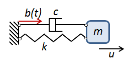 The SDOF system.
The equation of motion for the mass can, if there are no external forces, be written as

Dividing by the mass, and using customary notation,

Here, the undamped natural (angular) frequency is

and the damping ratio is

It can be seen that the support movement acts as a forcing term and that the solution depends only on the two parameters  and
and  , but not on the individual values of m, c, and k.
Instead of using the absolute displacement as the degree of freedom, it is possible to choose the relative displacement between the mass and the base,  . This is actually a frame transformation where the oscillator is studied in a coordinate system attached to the base. As in any accelerating frame, there will be inertial forces. The equation of motion can be stated as
 (1)
(1)
Thus, the support acceleration appears as a gravity-like load. There are two advantages with this representation:
- The internal forces in the system — that is, elastic and damping forces — depend on relative displacements and velocities. These forces are not affected by a rigid body motion.
- Often, measured data is available in terms of an accelerogram, so that the foundation displacements are not directly available.
For given values of , , and , this equation can be solved for a sufficiently long time. The displacement, velocity, and acceleration response spectra are defined as the maximum values caused by the acceleration history .



These are all relative spectra. It is possible to do a similar definition of the absolute spectra, by instead using the absolute displacement  .
.
Sometimes, a distinction is made between the positive and negative spectra, so that


and similarly for velocity and acceleration spectra.
The velocity and acceleration response spectra are often approximated by


Such spectra are called pseudovelocity and pseudoacceleration spectra.
For a system without damping, the pseudoacceleration spectrum based on the relative displacement is actually equal to the absolute acceleration spectrum. This can be seen from the undamped equation of motion,

Thus,

The maximum absolute value of the relative displacement must thus occur at the same time as the maximum absolute value of the absolute acceleration. The scale factor between the two is  . For systems with low damping, this relation will still be approximately true. Since most mechanical systems have a low damping (often 2% to 5%), it is customary to assume that the spectra for the absolute acceleration and the pseudoacceleration are the same.
Another common way of describing the damping in this context is by the Q factor (quality factor). The relation to the damping ratio is given by

How to Create a Response Spectrum
For a certain given time history, , a response spectrum is created in the following way:
- Select a frequency range for which the spectrum should be generated
- Select a frequency step that determines how many points on the response spectrum should be computed
- Select a certain damping ratio,
- For each of the selected frequencies
a. Solve Equation (1) with for a sufficiently long time
b. Keep track of the maximum value of and store it
The equation can be solved by a pure numerical time stepping, but there may be better ways of doing it. If  is given as a number of points in an accelerogram, then it is natural to assume that the acceleration has a linear variation in time between those points. So, for each interval between two measurements, say from
  to
to  , the equation of motion for the oscillator is

This equation, where the right-hand side is a linear function of time, can be solved analytically for each time interval. The initial conditions are obtained from the final state of the previous interval.
The maximum values can actually occur after the end of the driving event. This will happen for low values of (long periods). The time-stepping must thus be continued at least until a full period if the oscillator has elapsed.
With this formulation, it is possible to track the extreme values of the:
- Relative displacement
- Relative velocity
- Relative and absolute acceleration
The absolute displacement and velocity are not available, since only is known, but not  and . It is, of course, possible to recover the foundation velocity and displacement by time integration of the acceleration. In practice, this integration will, however, cause a drift, so that the final velocity and displacement turn out to be nonzero. Since nonzero final displacements and velocities are unphysical (at least for many types of events), some numerical filtering has to be applied. For shocks, there is also a question of which initial values should be chosen for the displacement and velocity of the foundation.
Example 1: A Half Sine Shock
A common description of impact, used in several standards, is a half sine acceleration pulse. The acceleration amplitude, as well as the duration of the shock, can have different values. The acceleration may, for example, be 20 g, 50 g, or 100 g (g = 9.8 m/s2), and the time of duration can be 6 ms or 11 ms. In this example, a 50-g half sine pulse with a duration of 11 ms is used as the acceleration .
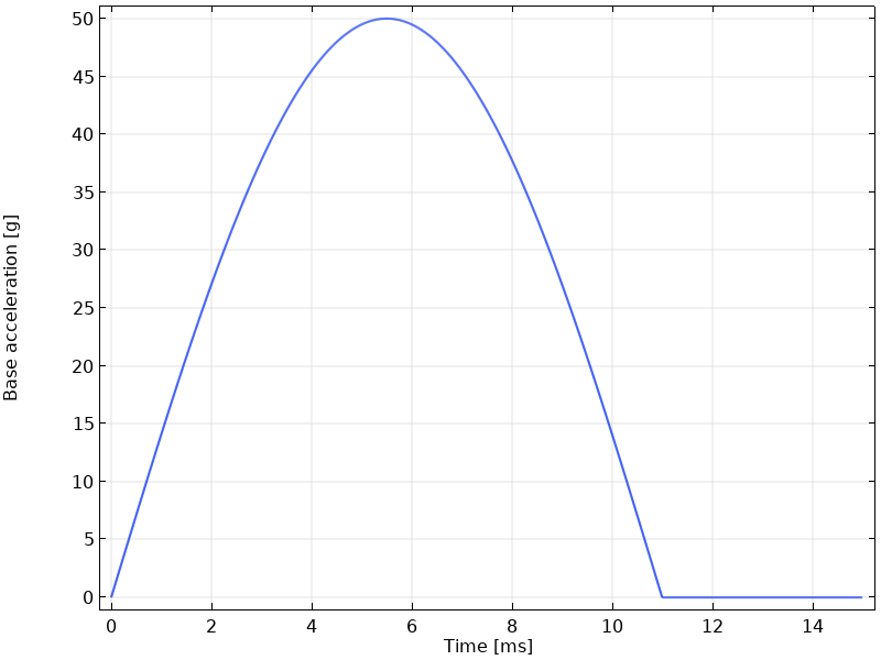 The base acceleration for the 50-g, 11-ms half sine shock.
The computed response spectra for 5% damping (Q = 10) is shown below.
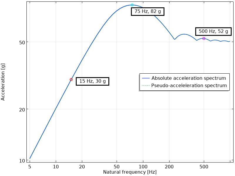 The absolute acceleration response spectrum for 5% damping plotted together with the corresponding pseudoacceleration spectrum.
The absolute acceleration has a maximum at frequencies similar to the frequency content of the input signal. In this case, the peak is at 74 Hz (T = 13.5 ms). For high frequencies, the acceleration spectrum tends toward 50 g. This is a general observation for any signal: At high frequencies, the oscillator will behave as a rigid body, so the mass just follows the base motion. As an effect, the asymptotic value of the absolute acceleration spectrum always equals the peak base acceleration during the event.
For low frequencies, the acceleration tends toward zero with a rate that is inversely proportional to the frequency. With a very soft oscillator, the base movement will just compress the spring without significant movement of the mass.
It can also be seen that the pseudoacceleration spectrum in this case is almost indistinguishable from the actual absolute acceleration spectrum, even though the damping is 5%.
In the figures below, the time response for the oscillator is shown for three different choices of its natural frequency, corresponding to the markers in the response spectrum above.
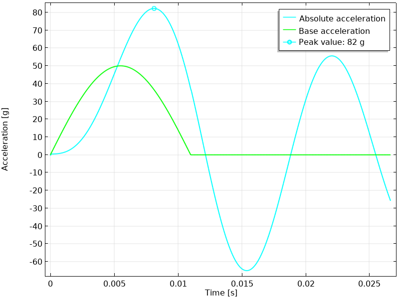
- At 15 Hz, the load pulse just gives a small initial push, and then the oscillator experiences free vibration at its natural frequency. The peak acceleration occurs a long time after the end of the excitation.
- At 75 Hz, there is maximum dynamic amplification. The load pulse is essentially in phase with the relative velocity, and it provides a maximal energy input to the system.
- At 500 Hz, the oscillator to a large extent acts as a rigid body, closely following the base acceleration. The peak acceleration is almost the same as that of the base acceleration.
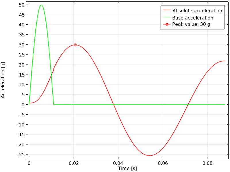 Absolute acceleration at a natural frequency of 15 Hz and damping of 5%.
 Absolute acceleration at a natural frequency of 75 Hz and damping of 5%.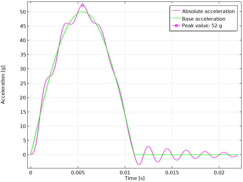
Absolute acceleration at a natural frequency of 500 Hz and damping of 5%.
The relative displacement spectrum is shown below. This is essentially the same as the acceleration spectrum above, but scaled with a factor 
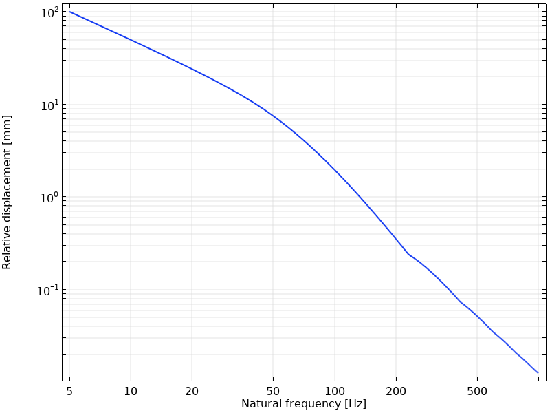 The relative displacement response spectrum for 5% damping.
Next, the relative velocity spectrum and the pseudovelocity spectrum are compared. As can be seen, they are quite different. The pseudovelocity and pseudoacceleration spectra do not represent the true relative spectra. This is a general observation, and the pseudo spectra should be viewed as different representations of the displacement spectrum.
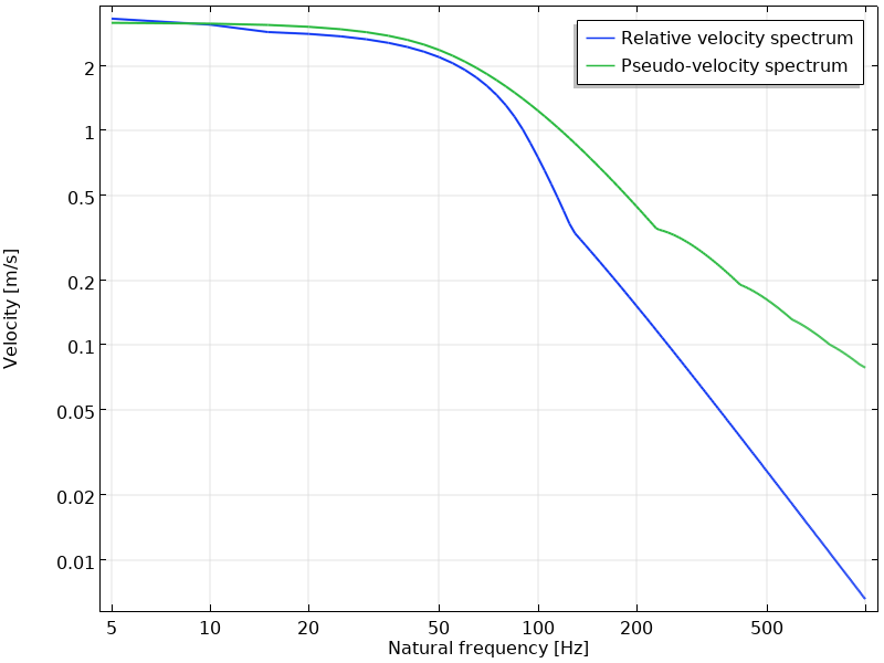 The relative velocity response spectrum and the pseudovelocity spectrum for 5% damping.
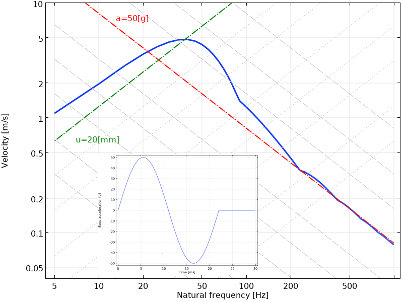
A convenient way to represent a response spectrum is in a tripartite, or four-axis plot. In such plot, the relative displacement, pseudovelocity, and pseudoacceleration are shown simultaneously. This is possible, since they are related by a factor of frequency and frequency squared, respectively, which in a logarithmic plot just gives lines with different slopes. The tripartite plot is essentially a pseudovelocity plot but with two extra sets of skewed grid lines that represent the displacement and acceleration, respectively.
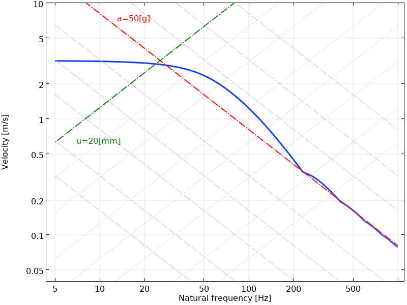 Tripartite plot of the response spectrum for the half sine pulse. The 50-g acceleration level and 20-mm displacement level are highlighted in red and green, respectively. The diagonal displacement (dotted) and acceleration (dashed) levels have the same '1-2-5-10' spacing as used for the velocity axis.
The response spectrum for the half sine pulse is actually somewhat atypical. The reason is that this pulse only has positive acceleration. If it is integrated with respect to time, such pulse corresponds to a resulting nonzero velocity and an ever-increasing displacement. Most events, like earthquakes, have the property that both displacement and velocity are zero both before and after the event. If a complete sine pulse is used instead of a half sine pulse, the characteristic low-frequency decay is also obtained.