Structural dynamics

1A)

Static Analysis

• The load remains constant with respect time.
• There might be slight motion in the object which can be neglected.
• The forces applied on the object are very slow with time hence the variation of loads with respect to time are neglected.
• The force that is accounted in this analysis is elastic force.
• Require more degree of freedom to find out stiffness of the structure as the displacement U in the structure is not noticeable (Required minimum 3 degree of freedom that is lateral force and 2 rotational forces.)

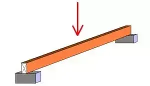
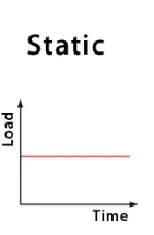
Fig A Example for static analysis

In fig A it is noticed a point load is acting on the beam where there will no changes in load with respect to time as shown in the graph.

Dynamic Analysis

• The load varies with respect to time, as the loads applied are very quick
• The motion in this analysis cannot be disregared due to which additional to elastic force, inertia force and damp force are accounted.
• Require less degree of freedom to find out stiffness of the structure. This is the displacement in the structure are noticeable and with the help of the displacement the stiffnesss of the strucutre are calculated.

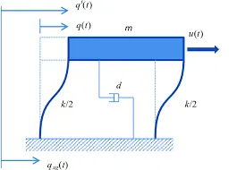
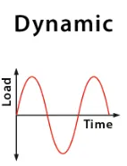
Fig B Example for dynamic analysis structure

In fig B it is noticed that a lateral force is applied to the structrue and released to oscilate. From the graph we can see that the load varies with time.

A2)

Elastic behaviour: It is a behaviour of the material which is having the ability to return to its original form (do not deform) when the material is away from the external force. Eg: Rubber band is the best example of elastic behaviour material. For linear system force can be expressed as fs=ku where k is lateral stiffness constant.

Inelastic behaviour: It is a behaviour of the material which is unable to return to its original form i.e it remains in deformed shape even after removal after external force. Eg Clay.

Plastic behaviour: It is behaviour of a material whose shapes remain deform and strains remain permanent after the yeild point even after removal of the load. Later this same material when external force increased will split at one particular point. Fig A represents the graphical representation of stress-strain.

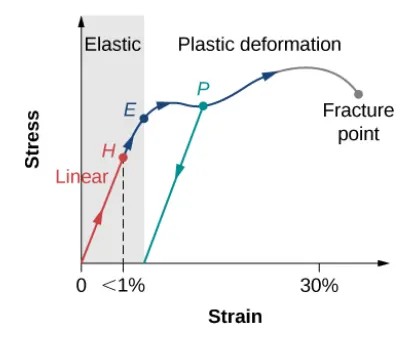
Fig C: Graphical representation of stress and strain curve.

Non-linear Inelastic behaviour: This behaviour in the material occur during large deforamtion where the material experience non linear loading and unloading forces in a cylic form. For non linear system force can be expressed as fs=fs(u,v). The Fig b shows the Force displacement relationship of the Non-linear inelastic behaviour. We can see in the curve that at initial point the loading is linear at later becomes non-linear and starts unloading (Point A-B-C) and again begins loading (Point C-D-A) but in the different path.

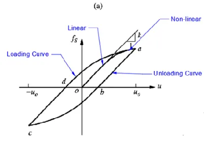
Fig D: Force displacement relationship of Non-Linear Inelastic behaviour

A3)

Mass component: In equation of motion the mass components considers only the mass of the structure and stiffness and damping are neglected. The force is related with mass component with the equation of fi=mu¨.

Stiffness component: Here stiffness is said to be the rigidity of a material to avoid deformation and in equation of motion the force related to stiffness is considered in the structure and other forces such as mass and damping are neglected. The equation for stiffness component is expressed as fs=ku.

Damping component: Damping is the inert force of the structure that helps dissipate the energy caused due to external force by vibrations over time and distances. It occurs due to the friction between structural and non stuctural elements, opening and closing of microcracks and friction at steel structures. The equation for stiffness component is expressed as fd=cu˙

Hence the equation of motion can be written as

mu¨+ fd + fs = p(t) that is mu¨ + cu˙ + ku = p(t) where p(t) is the external force.

A4)

Natural period: The time taken for undamped system to complete one cycle of free vibration is called as the natural period of vibration and the equation is expressed as Tn = 2π/ωn, here ωn=`square root`of K/m and the unit is seconds.

Natural frequency: The natural frequency is defined as the number of cycles i.e one full cycle of free vibration completed in one second. It is denoted in radians/sec.

The relation between and natural period and natural frequency is that frequency is inversely propotional to the period of vibration.

fn=1/Tn.

A5)

Response spectrum:

• It is a central concept of earthquake engineering of characterizing the ground motion and their effects on structures of different natural time period Tn.
• This concept helps us to summarise the peak response of all possible linear SDF system to a particular component of ground motion, conveniently and also helps us to apply this practical knowledge of structural dynamics to the design of structural and development of lateral force requirements in building codes.
• A peak value of the response spectrum can be obtained by plotting the response quantity of Displacement (u), Velocity (v) and Acceleration (a) of a response spectrum as a function of natural vibration period Tn. Each such plot is for the SDF system having fixed damping rotio and every such plot have different value of damping ratio are included to cover the range of damping values encountered in actual structures.
• This response spectrum can be of 3 type they are:
  • The deformation response spectrum- It is a plot of peak displacement (u) against natural period of time (Tn) with fixed dampness.
  • Relative velocity response spectrum- It is a plot of peak relative displacement.
  • Acceleration response spectrum- It is a plot of peak total displacement.

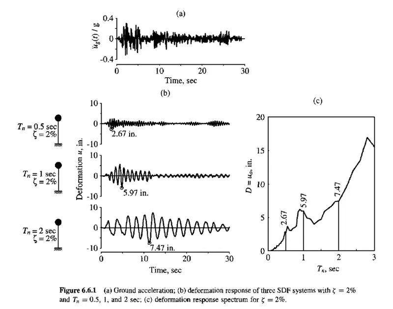
The Fig 6.6.1 shows the plot of deformation response spectrum of having a plot with deformation with respect to time . In this fig, the 1st plot (a) represents the ground motion recorded during a earthquake. The second plot (b) represents the plots of deformation respone of three different SDF systems. Each plots of b has been done with fixed damping ratio as 2% and variation in natural time period as 0.5s,1s,2s and the corresponding deformations are obtained with respect to time. With the help of the plot (b) a plot (c) of recorded deformation and Tn is obtained to record the peak responses. Based on these plots different structure can be designed.

Pseudo acceleration response spectrum:

• Pseudo acceleration for a single degree of freedom system with natural frequency ωn is related to its peak deformation D = uo, due to earthquake ground motion and it's equation is expressed as

A = (ωn^2) * D = ((2π/Tn)^2) * D.

• Since the D here represents the relative displacement and not the total displace, hence it is called Pseudo acceleration response spectrum, so to avoid confusion with acceleration response spectrum.
• The quantity A has units of acceleration and it is related with base shear Vbo. The equation is expressed as

Vbo = fso = mA (or) Vbo = (A/g)*ω.

• In this formula A/g is base shear coefficient where A is acceleration and g is gravitational force.

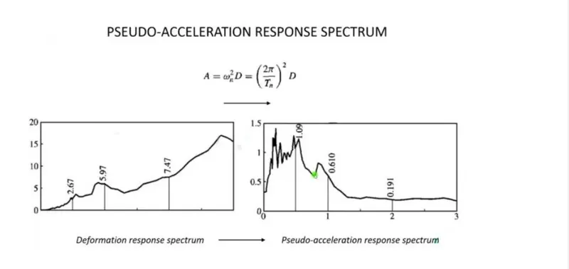
Fig E: Graphical difference between Deformation response spectrum and Pseudo-acceleration response spectrum

Fig E shows the defference between Deformation response spectrum and Pseudo acceleration response spectrum graph for the same structure having same ground motion. We can see that the in deformation respons spectrum that the Deformation is at peak at increase of natural period of time and where as in Pseudo acceleration response spectrum the deformation is at peak at low natural frequency and decline as the time period increases.