Steady vs unsteady state analysis
Objective:
Compare the convergence rate [Number of iterations] of the steady state and transient [explicit and implicit] simulations and justify the numerics.
Input:
Boundary conditions:
Top Boundary = 600 K
Bottom Boundary = 900 K
Left Boundary = 400 K
Right Boundary = 800 K
Error Criteria = 1e-4
STEADY STATE:
To define a steady state for a system, you’d observe that whatever affects the system’s behaviour are constant or unchanging in time Also, in terms of continuous-time, this means that for those properties of the system, the partial derivative in regards to time remains zero.
For our analysis we have to solve 2D heat conduction problem. Steady state for the problem can be defined as-
δ2Tδx2+δ2Tδy2=0
TRANSIENT STATE:
A transient state is essentially the time between the beginning of the event and the steady state.
Transient state can be defined by stating that if a quantity is at rest and a change in time takes place, thus changing the current state, a transient has occurred.
δTδt=α⋅(δ2Tδx2+δ2Tδy2)
JACOBI ITERATION METHOD:
In numerical linear algebra, the Jacobi method is an iterative algorithm for determining the solutions of a strictly diagonally dominant system of linear equations. Each diagonal element is solved for, and an approximate value is plugged in. The process is then iterated until it converges.
The formula for Jacobi Method for Steady State can be written as:
T(i,j)=(1k)⋅Told(i−1,j)+Told(i+1,j)Δx2+(1k)⋅Told(i,j−1)+Told(i,j+1)Δy2
where k=2⋅Δx2+Δy2Δx2⋅Δy2
; Told
is last iteration's value.
The formula for Jacobi Method for Transient Implicit State can be written as:
T(i,j)n+1=term1⋅Tprev(i,j)n+term2⋅(Told(i−1,j)n+1+Told(i+1,j)n+1)+term3⋅(Told(i,j−1)n+1+Told(i,j+1)n+1)
where k1=α.ΔTΔx2
; k2=α.ΔTΔy2 ; term1=11+2k1+2k2 ; term2=k1⋅term1 ; term3=k2⋅term1;Told is last iteration's value.; Tprev
is last Time Step's value; the value n and n+1, gives the time step
GAUSS-SEIDEL ITERATION METHOD:
Gauss–Seidel method is an iterative method to solve a set of linear equations and very much similar to Jacobi’s method.
Here the better solution is x = (x1, x2, … , xn), if x1(k+1) is a better approximation to the value of x1 than x1(k) is, then it would better that we have found the new value x1(k+1) to use it (rather than the old value that isx1(k)) in finding x2(k+1), … , xn(k+1). So x1(k+1) is found as in Jacobi’s Method, but in finding x2(k+1), instead of using the old value of x1(k) and old values of x3(k),…, xn(k), we then use the new value x1(k+1) and the old values x3(k), … , xn(k), and similarly for finding x3(k+1), … , xn(k+1)
The formula for Gauss-Seidel Method for Steady State can be written as:
T(i,j)=(1k)⋅T(i−1,j)+T(i+1,j)Δx2+(1k)⋅T(i,j−1)+T(i,j+1)Δy2
where k=2⋅Δx2+Δy2Δx2⋅Δy2
; Told
is last iteration's value.
The formula for Transient Implicit State can be written as:
T(i,j)n+1=term1⋅Tprev(i,j)n+term2⋅(T(i−1,j)n+1+T(i+1,j)n+1)+term3⋅(T(i,j−1)n+1+T(i,j+1)n+1)
where k1=α.ΔTΔx2
; k2=α.ΔTΔy2 ; term1=11+2k1+2k2 ; term2=k1⋅term1 ; term3=k2⋅term1;Told is last iteration's value.; Tprev
is last Time Step's value; the value n and n+1, gives the time step
SUCCESSIVE OVER RELAXATION ITERATION METHOD:
The method of successive over-relaxation (SOR) is a variant of the Gauss–Seidel method for solving a linear system of equations, resulting in faster convergence.
For any iterative method, in finding x(k+1) from x(k), we move a certain amount in a particular direction from x(k) to x(k+1). This direction is the vector x(k+1) − x(k), since x(k+1) = x(k) + (x(k+1) − x(k)). If we assume that the direction from x(k) to x(k+1) is taking us closer, but not all the way, to the true solution x , then it would make sense to move in the same direction x(k+1) − x(k), but farther along that direction.
SOR Method uses the value from Gauss Seidel to converge the results faster with a parameter ω
TSOR(i,j)=(1−ω)⋅Told(i,j)+ω⋅TGS(i,j)
For ω>1 we have Over-Relaxation and ω<1 we have Under-Relaxation.
EXPLICIT METHOD:
In the code used we can see the Explicit Approach used in the Transient Solutions:
Tn+1i,j=Tni,j+(α⋅Δt)(Tni+1,j−2⋅Tni,j+Tni−1,jΔx2+Tni,j+1−2⋅Tni,j+Tni,j−1Δy2)
Here the only term to be found out is the Tn+1i,j
, all the other terms used are from previous time steps, which are already known. Therefore, this equation can be solved explicitly and hence the name- Explicit Method.
IMPLICIT METHOD:
Referring to the equations noted earlier for the Jacobi, GS and SOR method we can see the Implicit method employed in the Transient Approach to solve the problem.
By definition, an implicit approach is one where the unknowns must be obtained by means of a simultaneous solution of the difference equations applied at all the grid points arrayed at a time level. Because of this need to solve large systems of simultaneous algebraic equations, implicit methods are usually involved with the manipulations of large matrices.
WHY IS STEADY STATE ANALYSIS FASTER THAN TRANSIENT STATE ANALYSIS:
Referring the above various definitions for Steady State and Transient State analysis for both Explicit and Implicit analysis we can say-
- Steady State simulation computes the fully developed solution that does not change in time.
- Mean values are computed with Steady State.
- Steady-state simulations are faster than transient.
- Transient simulation computes the instantaneous values in each time for each quantity.
The results of transient simulation may be more comprehensive.
CODE FOR STEADY STATE:
%Solving the Steady State 2D heat conduction problem
clear all
close all
clc

%Defining GRID and INPUTS_GRID - 10*10 matrix
nx = 10;
ny = 10;
t = ones(nx, ny);
t(1:nx, 1)  = 400;
t(1, 1:ny)  = 600;
t(1:nx, ny) = 800;
t(nx, 1:ny) = 900;
t(1,1) = (t(1,2)+t(2,1))/2;             %Assigning Corner values
t(nx,1) = (t(nx-1,1)+t(nx,2))/2;        %Assigning Corner values
t(1,ny) = (t(1,ny-1)+t(2,ny))/2;        %Assigning Corner values
t(nx,ny) = (t(nx-1,ny)+t(nx,ny-1))/2;   %Assigning Corner values
t(2:nx-1,2:ny-1) = 300;                 %Assuming grid values

error = 9e9;
tolerance = 1e-4;
x = linspace(0,1,nx);
y = linspace(0,1,ny);
dx = 1/(nx-1);
dy = 1/(ny-1);
[xx yy] = meshgrid(x,y);
k = 2*(dx^2 + dy^2)/(dx^2 * dy^2);
told = t;
tinitial = t;
jacobi_iteration = 0;
gs_iteration = 0;
sor_iteration = 0;
w = 1.5;

%Selecting method to solve Steady State Problem
method = input('Select the method to solve the Steady State problem \n 1. Jacobi \n 2. Gauss-seidel \n 3. Successive over-relaxation \n')

%Code for JACOBI METHOD
if method==1
    while error>tolerance
        %Space Loop
        for i = 2:nx-1
            for j = 2:ny-1
                H = (told(i-1,j)+told(i+1,j))/(dx^2);
                V = (told(i,j-1)+told(i,j+1))/(dy^2);
                t(i,j) = (H+V)/k;
            end
        end
        diff = abs(told-t);
        error = max(max(diff));
        told = t;
        jacobi_iteration = jacobi_iteration +1;
    end
    fprintf('Number of Iterations for Jacobi Method = %d', jacobi_iteration)
    %Plot for JACOBI METHOD
    contourf(x,y,t,'showtext','on')
    colormap(jet)
    colorbar
    set(gca,'YDIR','reverse')
    xlabel('X axis')
    ylabel('Y axis')
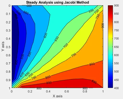
    title(sprintf('Steady Analysis using Jacobi Method'))
end


%Code for Gauss-seidel
if method==2
    while error>tolerance
        %Space Loop
        for i = 2:nx-1
            for j = 2:ny-1
                H = (t(i-1,j)+told(i+1,j))/(dx^2);
                V = (t(i,j-1)+told(i,j+1))/(dy^2);
                t(i,j) = (H+V)/k;
            end
        end
        diff = abs(told-t);
        error = max(max(diff));
        told = t;
        gs_iteration = gs_iteration +1;
    end
    fprintf('Number of Iterations for Gauss-Seidel Method = %d', gs_iteration)
    %Plot for Gauss-seidel
    contourf(x,y,t,'showtext','on')
    colormap(jet)
    colorbar
    set(gca,'YDIR','reverse')
    xlabel('X axis')
    ylabel('Y axis')
    title(sprintf('Steady Analysis using Gauss-seidel Method'))
end


%Code for Successive over-relaxation
if method==3
    while error>tolerance
        %Space Loop
        for i = 2:nx-1
            for j = 2:ny-1
                H = (t(i-1,j)+told(i+1,j))/(dx^2);
                V = (t(i,j-1)+told(i,j+1))/(dy^2);
                tgs(i,j) = (H+V)/k;
                t(i,j) = (1-w)*told(i,j) + w*tgs(i,j);
            end
        end
        diff = abs(told-t);
        error = max(max(diff));
        told = t;
        sor_iteration = sor_iteration +1;
    end
    fprintf('Number of Iterations for Successive over-relaxation method = %d', sor_iteration)
    %Plot for Successive over-relaxation
    contourf(x,y,t,'showtext','on')
    colormap(jet)
    colorbar

    set(gca,'YDIR','reverse')
    xlabel('X axis')
    ylabel('Y axis')
    title(sprintf('Steady Analysis using Successive Over Relaxation Method'))
end
OUTPUT:
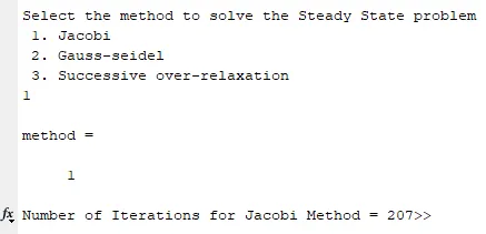
1. Jacobi Method
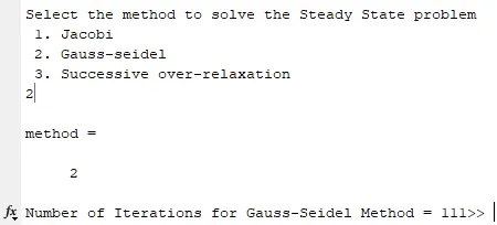
2. Gauss-Seidel Method
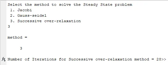
3. SOR Method
OUTPUT PLOTS:
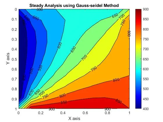
1. Jacobi Method
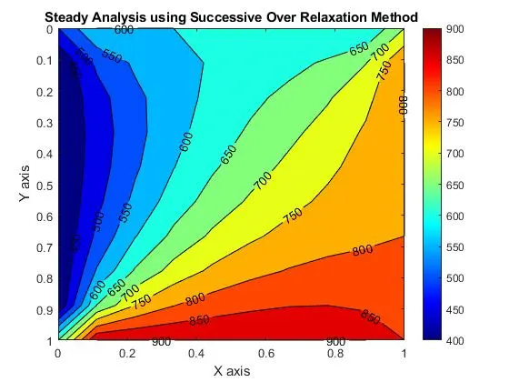
2. Gauss-Seidel Method
3. SOR Method
CODE FOR TRANSIENT STATE:
%Solving the Transient State 2D heat conduction problem
clear all
close all
clc

%Defining GRID and INPUTS_GRID - 10*10 matrix
nx = 10;
ny = 10;
t = ones(nx, ny);
t(1:nx, 1)  = 400;
t(1, 1:ny)  = 600;
t(1:nx, ny) = 800;
t(nx, 1:ny) = 900;
t(1,1) = (t(1,2)+t(2,1))/2;             %Assigning Corner values
t(nx,1) = (t(nx-1,1)+t(nx,2))/2;        %Assigning Corner values
t(1,ny) = (t(1,ny-1)+t(2,ny))/2;        %Assigning Corner values
t(nx,ny) = (t(nx-1,ny)+t(nx,ny-1))/2;   %Assigning Corner values
t(2:nx-1,2:ny-1) = 300;                 %Assuming grid values
told = t;
tprev = t;
error = 9e9;
tolerance = 1e-4;
x = linspace(0,1,nx);
y = linspace(0,1,ny);
dx = 1/(nx-1);
dy = 1/(ny-1);
[xx yy] = meshgrid(x,y);
dt = 1e-4;
iteratoin_explicit = 0;
alpha = 1.4;
k1 = (alpha*dt)/(dx^2);
k2 = (alpha*dt)/(dy^2);

%Selecting method to solve Transient State Problem
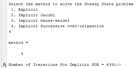
method = input('Select the method to solve the Steady State problem \n 1. Explicit \n 2. Implicit Jacobi \n 3. Implicit Gauss-seidel \n 4. Implicit Successive over-relaxation \n')

% For Explicit Method
if method == 1
    for nt = 1:1400
        for i = 2:nx-1
            for j = 2:ny-1
                t(i,j) = told(i,j) + k1*(told(i-1,j)-2*told(i,j)+told(i+1,j)) + k2*(told(i,j-1)-2*told(i,j)+told(i,j+1));
            end
        end
        told = t;

    end
    contourf(x,y,t,'showtext','on')
    colormap(jet)
    colorbar
    set(gca,'YDIR','reverse')
    xlabel('X axis')
    ylabel('Y axis')
    title(sprintf('Transient Analysis using Explicit Method'))
end


% For Implicit Jacobi Method
if method == 2
    iteration_implicit_jacobi = 1;
    term1 = 1/(1+2*k1+2*k2);
    term2 = k1*term1;
    term3 = k2*term1;
    for nt = 1:1400
        error = 9e9;
        while(error>tolerance)
            for i = 2:nx-1
                for j = 2:ny-1
                    H = told(i-1,j)+told(i+1,j);
                    V = told(i,j-1)+told(i,j+1);
                    t(i,j) = term1*tprev(i,j) + term2*H + term3*V;
                end
            end
            diff = abs(told-t);
            error = max(max(diff));
            told = t;
            iteration_implicit_jacobi = iteration_implicit_jacobi + 1;
        end
        tprev = t;
    end
    fprintf('Number of Iterations for Implicit Jacobi Method = %d', iteration_implicit_jacobi)
    contourf(x,y,t,'showtext','on')
    colormap(jet)
    colorbar
    set(gca,'YDIR','reverse')
    xlabel('X axis')
    ylabel('Y axis')
    title(sprintf('Transient Analysis using Implicit Jacobi Method'))
end

% For Implicit Gauss-Seidel Method
if method == 3
    iteration_implicit_GS = 1;
    term1 = 1/(1+2*k1+2*k2);
    term2 = k1*term1;
    term3 = k2*term1;
        for nt = 1:1400
            error  = 9e9;
            while(error>tolerance)
                for i = 2:nx-1
                    for j = 2:ny-1
                        H = t(i-1,j)+t(i+1,j);
                        V = t(i,j-1)+t(i,j+1);
                        t(i,j) = term1*tprev(i,j) + term2*H + term3*V;
                    end
                end
            iteration_implicit_GS = iteration_implicit_GS + 1;
            diff = abs(told-t);
            error = max(max(diff));
            told = t;
        end
    tprev = t;
    end
    fprintf('Number of Iterations for Implicit Gauss-Seidel Method = %d', iteration_implicit_GS)
    contourf(x,y,t,'showtext','on')
    colormap(jet)
    colorbar
    set(gca,'YDIR','reverse')
    xlabel('X axis')
    ylabel('Y axis')
    title(sprintf('Transient Analysis using Implicit Gauss-Seidel Method'))
end

% For Implicit SOR Method
if method == 4
    iteration_implicit_SOR = 1;
    term1 = 1/(1+2*k1+2*k2);
    term2 = k1*term1;
    term3 = k2*term1;
    w = 1.015;
    for nt = 1:1400
        error = 9e9;
        while(error>tolerance)
            for i = 2:nx-1
                for j = 2:ny-1
                    H = t(i-1,j)+t(i+1,j);
                    V = t(i,j-1)+t(i,j+1);
                    t(i,j) = term1*tprev(i,j) + term2*H + term3*V;
                    t(i,j) = (1-w)*told(i,j) + w*t(i,j);
                end
            end
            iteration_implicit_SOR = iteration_implicit_SOR + 1;
            diff = abs(told-t);
            error = max(max(diff));
            told = t;
        end
        tprev = t;
    end
    fprintf('Number of Iterations for Implicit SOR = %d', iteration_implicit_SOR)
    contourf(x,y,t,'showtext','on')
    colormap(jet)
    colorbar
    set(gca,'YDIR','reverse')
    xlabel('X axis')
    ylabel('Y axis')
    title(sprintf('Transient Analysis using Implicit SOR Method'))
end
OUTPUT:
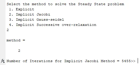
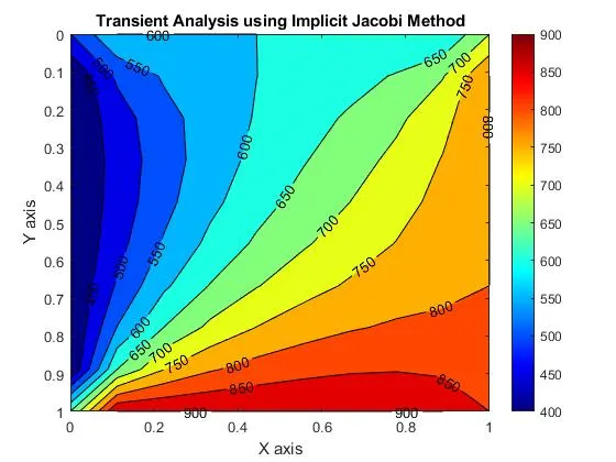
1. Implicit Jacobi Method
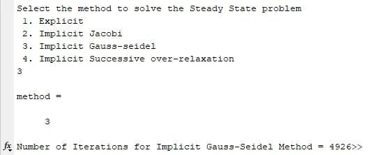
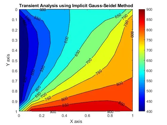
2. Implicit Gauss-Seidel Method
3. Implicit SOR Method
OUTPUT PLOTS:
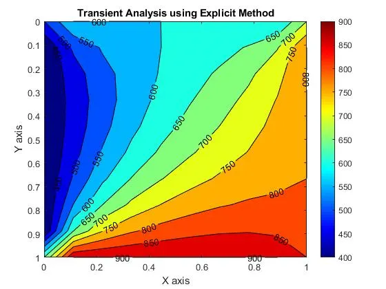
1. Explicit Method
2. Implicit Jacobi Method
3. Gauss-Seidel Method
4. SOR Method
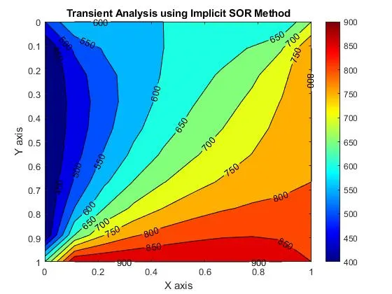
RESULT EXPLANATION:
It can be seen that for the Steady State there is significant drop in the number of iterations to converge the results from assumed values for following,
Jacobi (207) > Gauss-Seidel (111) > SOR(28).
For SOR the ω selected was 1.5. For ω value we can check for optimum value by trial and error method, which was employed here for the accuracy of 0.1 and found that 1.5 was optimum owing to its quicker iteration and convergence. Higher values for ω can lead to higher iterations and convergence time.
Similarly, for Transient Implicit State it can be seen that it follows similar trend,
Jacobi (5455) > Gauss-Seidel (4926) > SOR(4391).
From the above results, it can be said that the Steady State takes lower number of iterations when compared with the Transient methods.
For SOR the ω values selected is 1.015. For Transient Implicit Analysis it seems that the SOR is highly sensitive with the ω value as the iterations values starts increasing exponentially with the increase in ω value.