Steady Vs Unsteady flow over a cylinder

Abstract:

Flow past a cylinder is studied. the diameter of the cylinder is 2 meters. For Reynolds number 100, both steady and transient state simulation is carried out. Vortex shedding phenomenon is visualized. The relationship between vortex shedding and strouhal number is studied. Steady state analysis is carried out for the flow at various Reynolds number like 10,100,1000,10000,100000. the drag coefficient is calculated at all the reynolds number.

Key-words : Vortex shedding, Von-karman vortex street, reynolds number, Strouhal number, Drag Coefficient, Drag crisis.

Introduction:

The flow over a cylinder is a complex phenomenon and a matter of study still worldwide. At reynolds number less than 4, the flow is called creeping flow. At reynolds number between 10 and 40, two symmetrical vortices are visualized in the wake reginonof the cylinder. At reynolds number greatre than 40, Vortex shedding can be visualized.

In fluid dynamics vortex shedding is an oscillating flow that takes place when a fluid such as air or water flows past a bluff (as opposed to streamlined) body at certain velocities, depending on the size and shape of the body. In this flow, vortices are created at the back of the body and detach periodically from either side of the body forming aVon Karman vortex street The fluid flow past the object creates alternating low-pressure vortices on the downstream side of the object. The object will tend to move toward the low-pressure zone.

Reynolds number : It is a dimensionless number , represented by the ratio of inertia forces and the viscous forces.

Strouhal number : A dimensionless number represented by `(f*D)/V`. f is the frequency of the oscillation, D is the characteristic dimension and V is the free stream velocity.

Flow chart of the simulation:

• Geometry preparation using the Ansys spaceclaim
• Mesh generation using the ansys mesher
• Problem set up, initializing the boundary conditions, solver and the physics (pre-processing)
• Solution
• Post processing using CFD post

Geometry:

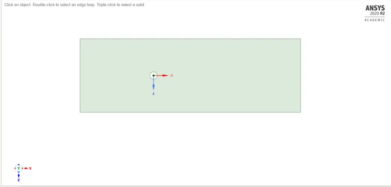
Ansys Spaceclaim is used to prepare the geometry. The diameter of the cylinder is 2 meters. The Domain is rectangular of length 60 meters and breadth 20 metrs. A 2D space is prepared for te study.

Meshing:

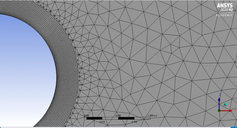
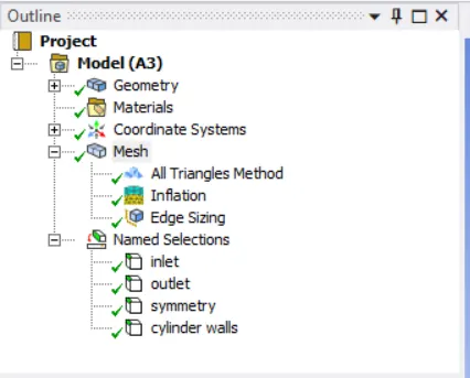
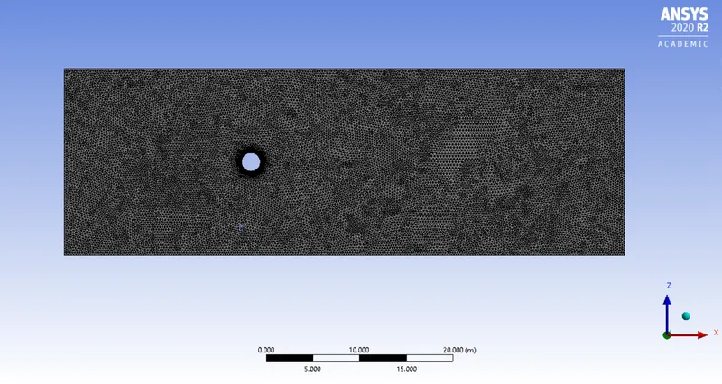
Meshing is one of the most important aspect of any CFD study. The default meshing that ansys mesher provides for the geometry is not satisfactory. The flow physics needs to be captured near the cylinder walls more rigorously. So inflation layers are added. The mesh is triangular. elememt size is 0.25. Named selections are provided to initialize the boundary conditions. The edge selection tool is enabled and then edges are selected one by one to provide the named selections.

To check the mesh quality, the mesh metrics is checked.

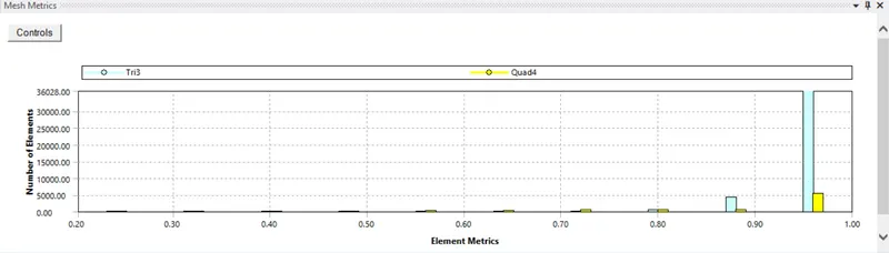
since the mesh metric shows most of the lements is above thw 90% catagory. The mesh is pretty good and the physics should be captured well.

Number of cells = 47946

Set-up:

Parallel system with 6 processors and 2 GGPU s are selected.

The formula to find out Reynolds number is given by Re= `(rho*V*D)/(mu)`

here `rho`is the density of the fluid, `V`is the velocity of the incoming fluid stream `D`is the characteristic dimension and `mu`is the dynamic viscosity of the fluid.

In the study flow at different Reynolds number is studied. The Reynolds number can be variedby two ways , one by increasing the velocity of the incoming fluid or by decreasing the dynamic viscosity of the fluid. Since for a fluid , The dynamic viscosity is constant. The Reynolds number is varied by varying the incoming velocity of the fluid.

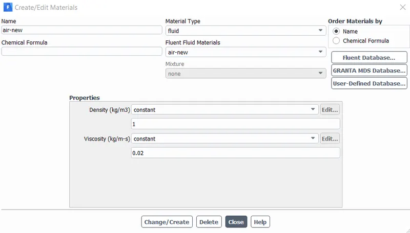
the material is created a hypothetical one with density =1 and the viscosity as 0.02 as constant.

• Reynolds Number 100, steady flow:

The solver selected is pressure based solver. Steady flow is studied. The velocity format selected is Absolute.

A monitor point is created at an distance of 8 meter from the center of the cylinder wall. the flow parameters will be studied at the monitor point.

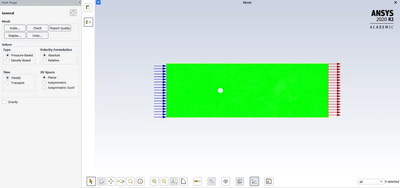
The boundary conditions are the inlet,outlet,the symmetry surfaces, cylinder walls , and the interior fff surface that ansys creates by default.

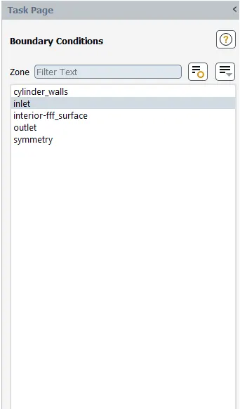
For the inlet, it is avelocity boundary, the free stream velocity is set up here. The velocity of the incoming fluid is 1 (m/s). the velocity direction is normal to the boundary.

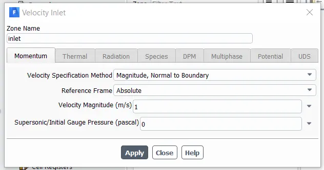
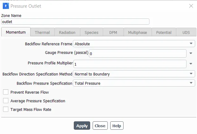
The outlet is being assigned with pressure based boundary condition and thats bydefault ansys does. The pressure is 0 pa (gauge pressure)

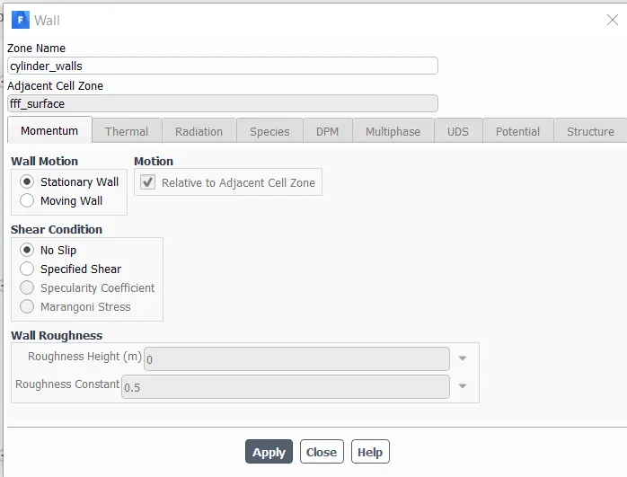
The cylinder walls are stationary walls with no slip condition enabled.

The initializaion is hybrid and the number of iterations set is 800.

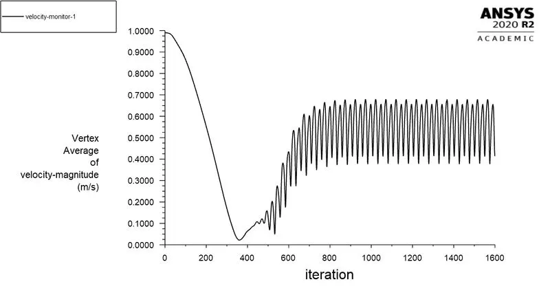
The velocity profile at the monitor point is :

The contour of the velocity distribution along all the boundary points is created after the initialisation is done.

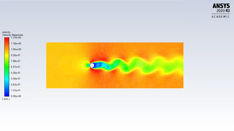
The vortex shedding phenomenon is visible from the simulation.

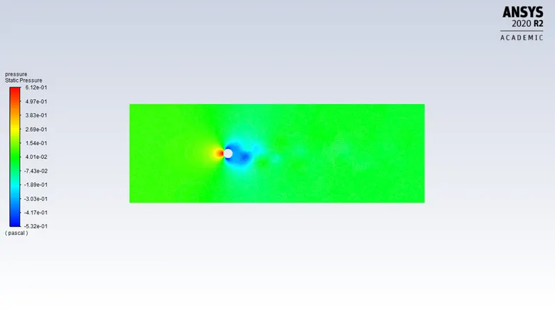
The pressure profile is :

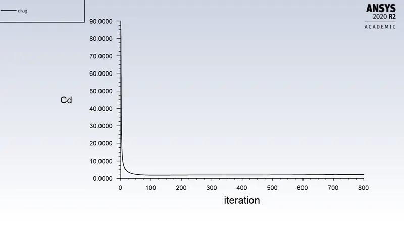
Plot showing the drag coefficient at the cylinder walls:

Coefficient of drag =2.194

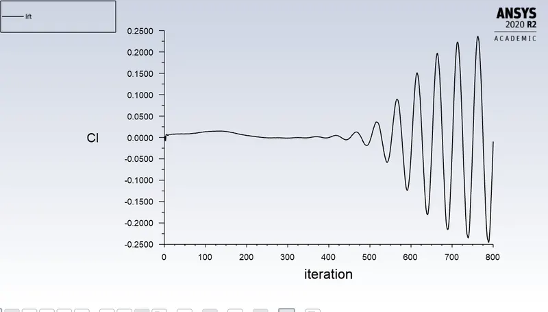
The coefficient of lift plot :

Velocity profile at monitor pint:

• Reynolds number 100, transient state:

To simulate the flow for the transient state , the pressure based solver is used. Standard initialization is followed and other parametrs are same.

The time step size is 0.1 s and the number of time steps is 1000.

the scaled residuals, the drag coefficient and the lift coefficient polts are:

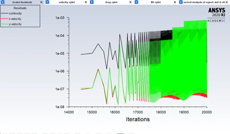
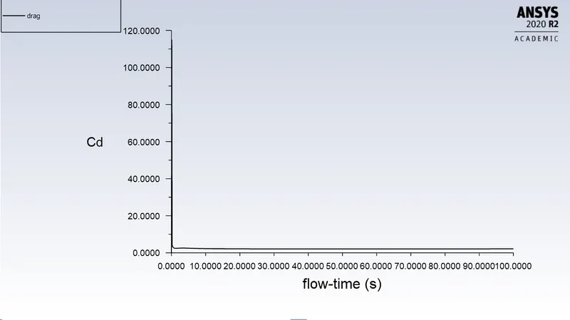
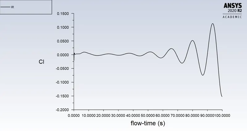
since it is transient study, the x axis is flow time.

The velocity and pressure contour are:

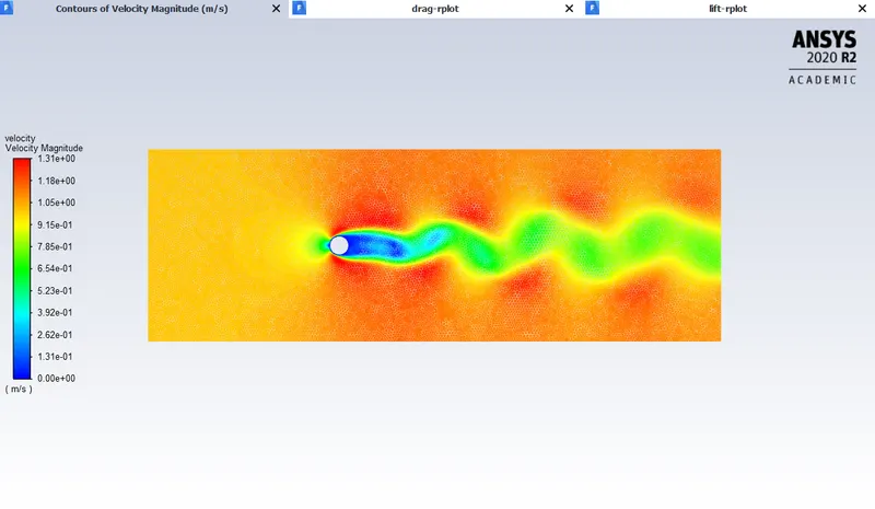
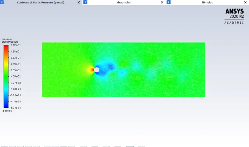
Vortex shedding can be noticed from the above contours.

The strouhal number is plotted against the magnitude

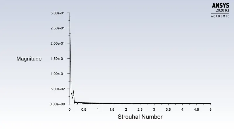
when the strouhal number is 0.17 the solution converges.

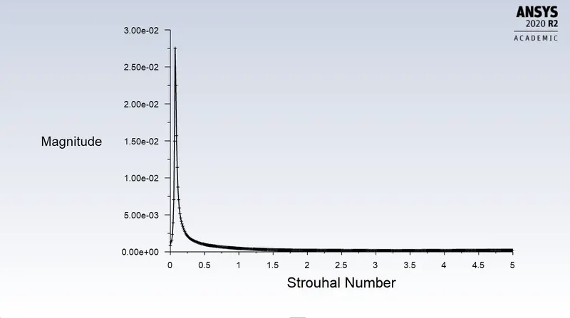
From the plot above it can be said that the maximum lift occurs when the Strouhal number is 0.17

The coefficient of drag and the coefficient of lift calcukated is :

Cd= 2.1441148

• Reynolds number =10, steady state:

The reynolds number is manipulated by manipulating the free stream velocity of the fluid considered. All other parameters are same. Number of iteretaions set is 800. The velocity profile, drag coefficient,lift coefficient and the pressure and velocity contours are studied. Since the Reynolds number is pretty low , the vortex shedding phenomenon do not takes place . Since reynolds number is too low, laminar model is chosen

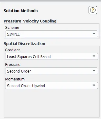
Pressure based solver , steady state analysis and the simple scheme is selected.

The boundary conditions are :

For the inlet, the free stream velocity is 0.1(m/s).

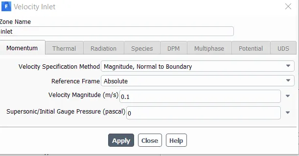
All the other boundary conditions are same as the before.

The Solution method chosen is shown below:

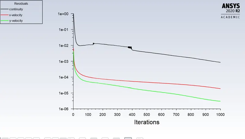
The sacled residuals after 1000 iterations are:

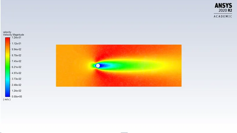
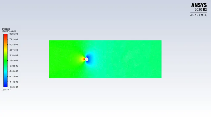
The velocity and pressure contours are respectively:

The velocity , drag and lift profiles are:

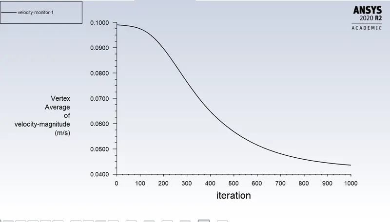
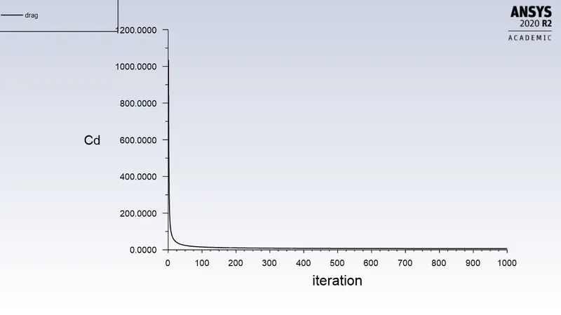
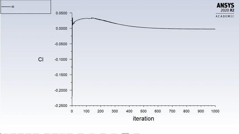
The coefficient of drag calculated is : = 6.7675871

The vortex shedding phenomenon is not noticed for the reynolds number so less . For Reynolds number between 10 and 40, two small steady eddies appear behind the cylinder and form a closed separation zone contained with a separation streamline. This zone is sometimes called a separation bubble. The cylinder's wake is completely laminar and the vortices rotate in a manner that is consistent with the exterior flow. These eddies grow in length and width as Re increases.

• Reynolds number = 1000, steady state :

The free stream velocity is increased to 10 (m/s). All other parameters are same.

As the reynolds number is still within the limits of laminar flow .

Pressure based solver and steady state is selected. Hybrid initialized.

1000 iterations are done.

The scaled residuals are as follows:

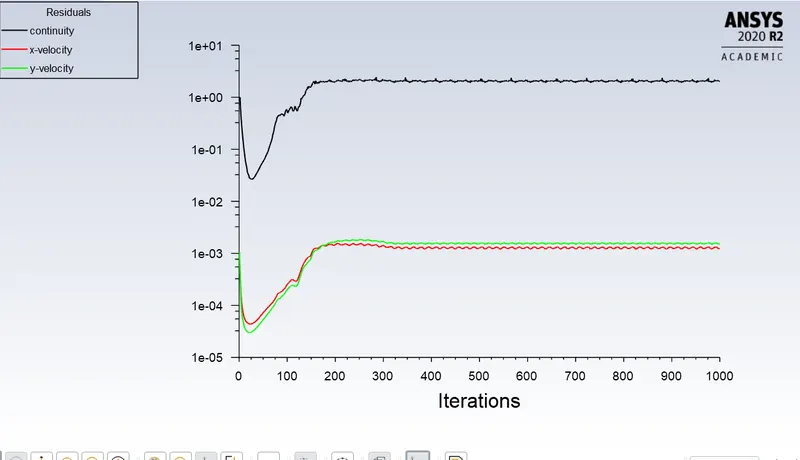
This shows that the solutions converged nearly after 200 iterations.

The velocity profile at the monitor plot is :

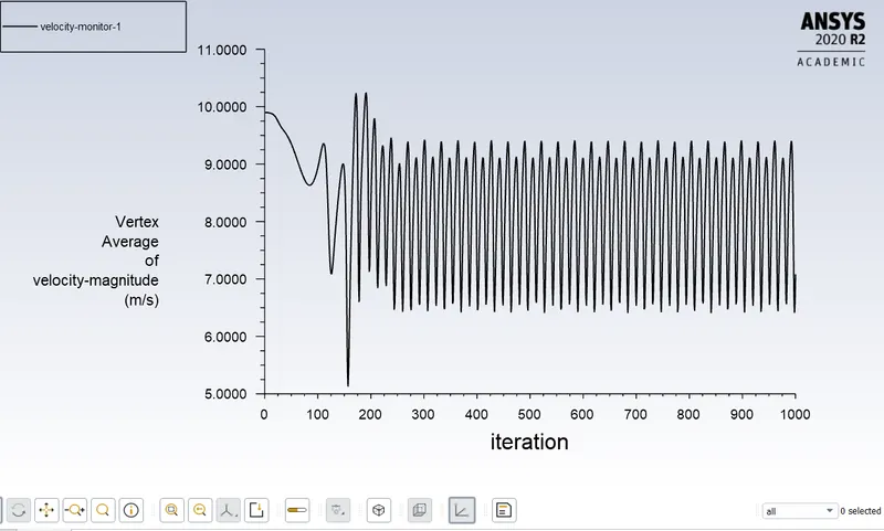
From the above plot it can be inferred that the vortex shedding phenonmenon takes place.

The drag coefficient and the lift coefficient can be plotted as :

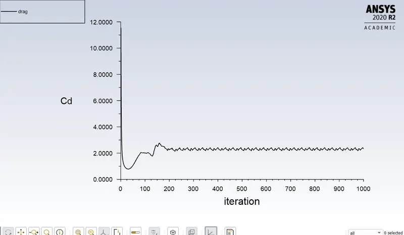
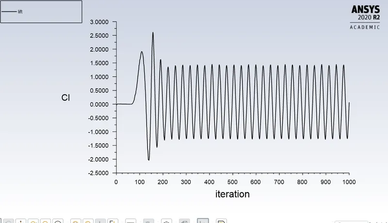
The drag and lift coefficient calculated are :

Coefficient of drag = 2.3239429

Coefficient of lift = 0.067852702

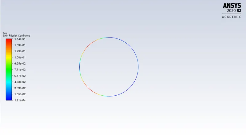
The velocity, pressure and the skin friction contours are:

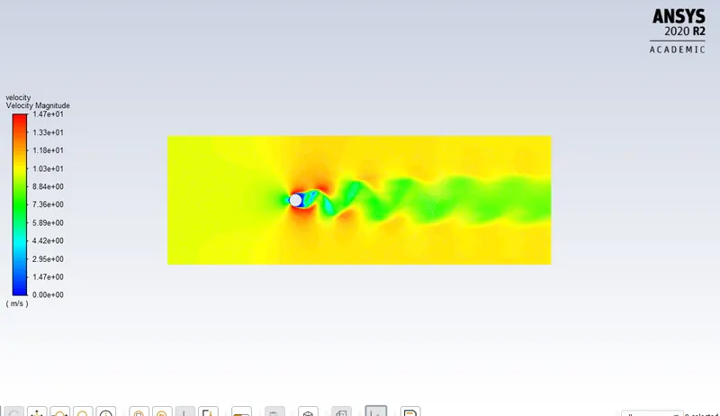
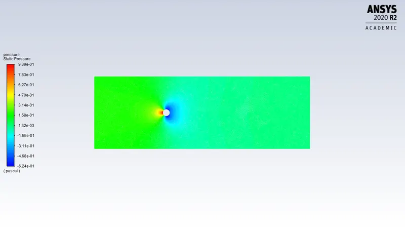
The Von Karman vortex street formation is visulaised from the velocity contour.

• Reynolds number = 10,000, steady state :

The free stream velocity at the inlet is 100 (m/s)

As the Reynolds number has crossed the limits of laminar flow , Turbukence model is selected the turbulence model selected is realizable K-Epsilon turbulence model with standard wall functions.

Pressure based solver and steady state is selected.

All other parameters are same.

Number of iterations set = 1000

The scaled residulas plot:

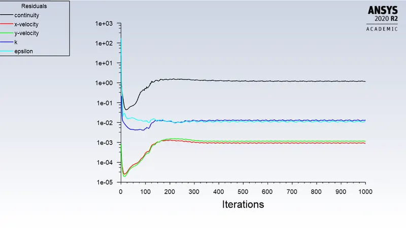
At around 180 iterations the solutions converged.

The velocity profile at the monitor point is:

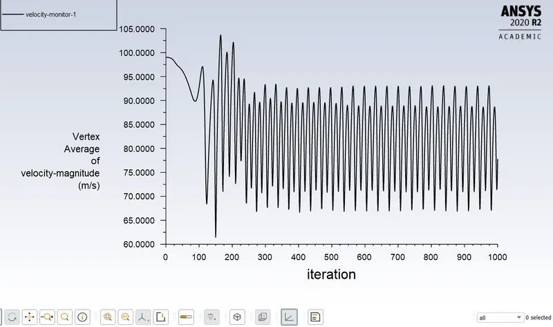
The drag coefficiemt and the lift coefiicient are:

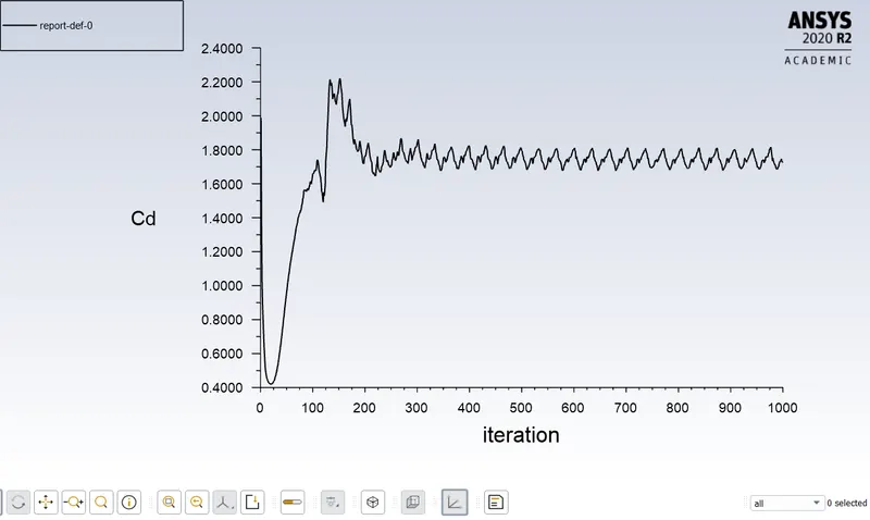
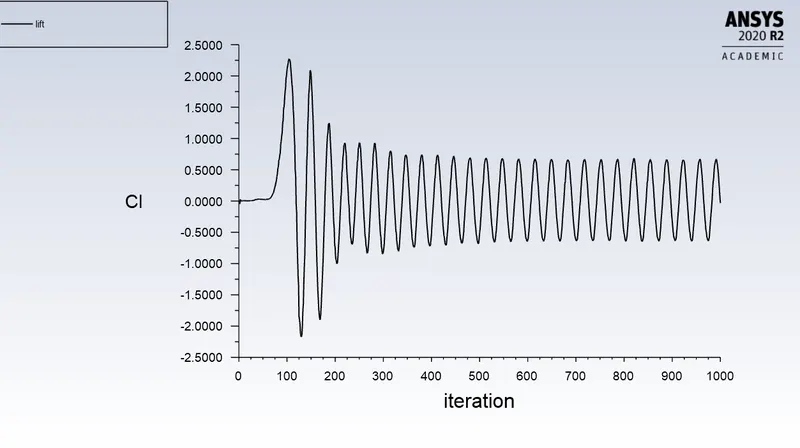
The coefficient of drag and coefficient of lift calculated is :

The drag coefficient is = 1.7293952

The velocity,pressure contours and skin fric around the cylindr walls are:

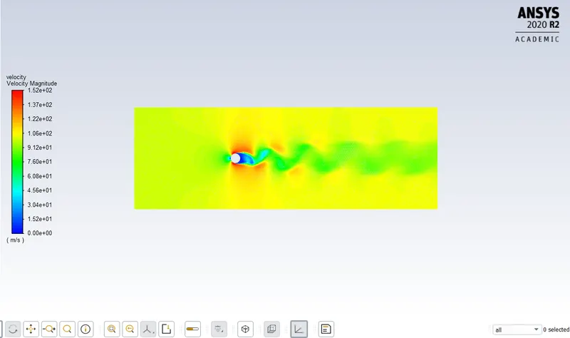
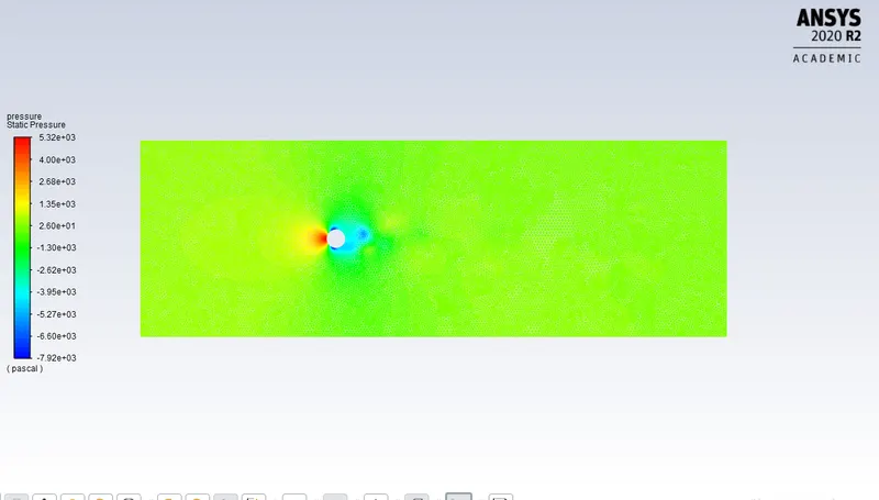
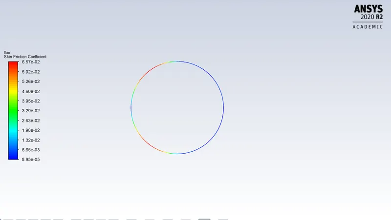
From the velocity contour, the Von Karman vortex street can be visualized.

• Reynolds number 100000, steady state:

The free stream velocity at the inlet is increased to 1000 (m/s).

At such high reynolds number, realizable K-epsilon turbulence model with standard wall functions is selected for the turbulence modelling.

Pressure based solver is selected. Steady stae is selected.

All other operating conditions and boundary conditions are same.

number of iterations = 1000

The scaled residuals are:

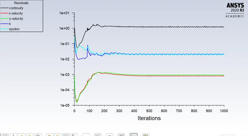
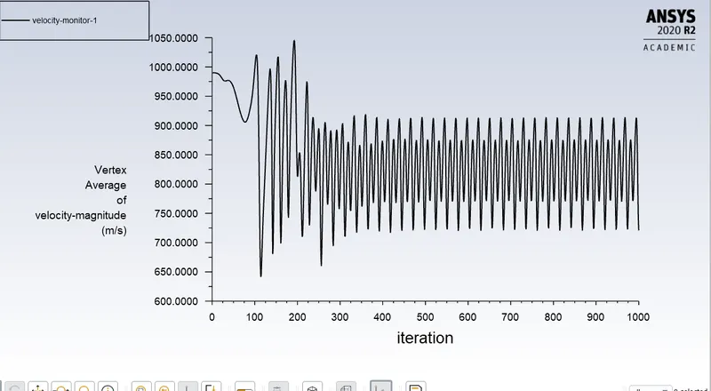
The velocity at the monitor point is:

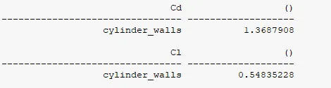
The coefficent of drag and coefficient of lift are :

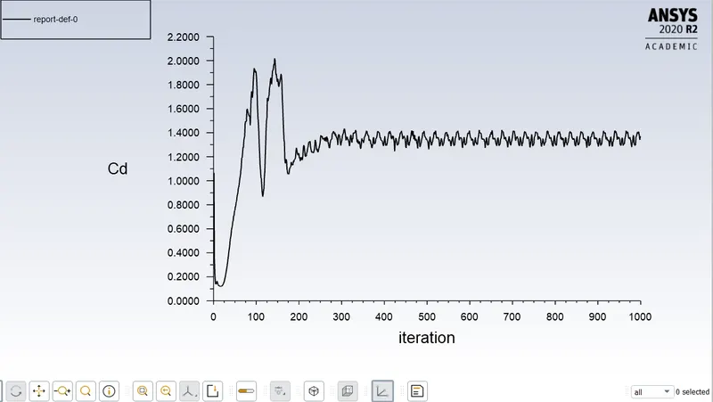
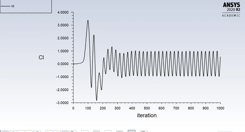
The drag coefficient and the coefficient of lift calculated are:

The velocity contour, pressure contour and the skin friction around the cylinder wall are:

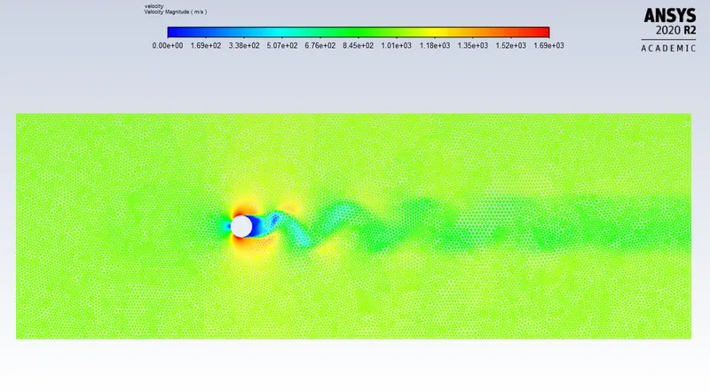
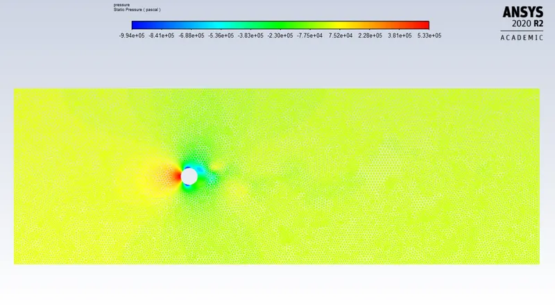
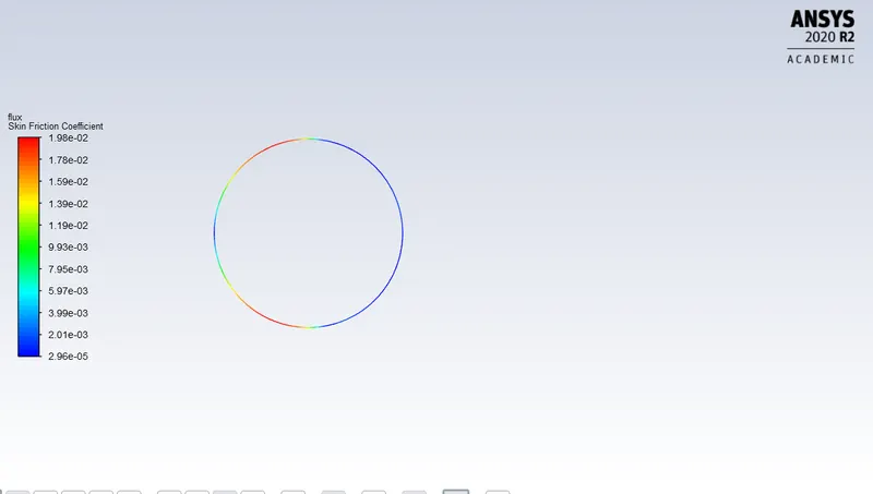
The vortex shedding phenomenon can be visualized.

Inference:

Comparison of coefficient of drag at various Reynolds number:

Reynolds Number	Coefficient of Drag
10	6.7675
100	2.1945
1000	2.3239
10000	1.7293
100000	1.3687

It is seen that with the increse in Reynolds number the drag coefficient decreases.

1. The drag coefficient decreases at low Reynolds numbers because the flow is in a regime called creeping flow. Creeping flow is visualized when the Reynolds number is less than 4 That is, the inertial forces are negligible. In this region, the Reynolds number isn't all that great of a parameter for the drag coefficient because the governing equations are independent of the Reynolds number. In spite of this, it is possible to analytically find the drag coefficient at very low Reynolds number to be inversely proprtional to reynolds number Once the drag coefficient levels off, the flow is now in the laminar region with significant inertial effects.

2. The large dive in the drag coefficient is called the drag crisis. This happens when the boundary layer over the cylinder transitions from laminar to turbulent. Turbulent boundary layers are more resistant to separation, so the flow stays attached longer resulting in decreased form drag.