Steady Vs Unsteady flow over a cylinder
Problem Definition
We have to simulate the flow over a cylinder and explain the phenomenon of Karman vortex street.
We have to calculate simulate for the following cases:-
1. Simulate the flow with the steady and unsteady case and calculate the Strouhal Number for Re= 100
2. Calculate the coefficient of drag and lift over a cylinder by setting the Reynolds number to 10,100,1000,10000 & 100000. (Run with steady solver)
Introduction
Karman vortex street
The Karman vortex street is an exquisite flow pattern that can be seen in a variety of flow situations. Karman vortex street is a repeating pattern of swirling vortices, caused by a process known as vortex shedding, which is responsible for the unsteady separation of flow of fluid around blunt bodies. A very interesting sequence of events begins to develop when the Reynolds number is increased beyond 48, at which the wake behind the cylinder becomes unstable. The wake develops a slow oscillation in which the velocity is periodic in time and in the downstream direction. The amplitude of the oscillation increases in the downstream direction. The oscillating wake rolls up into two staggered rows of vortices with opposite sense of rotation
vortex shedding is an oscillating flow that takes place when a fluid such as air or water flows past a bluff (as opposed to streamlined) body at certain velocities, depending on the size and shape of the body. A vortex street will form only at a certain range of flow velocities, specified by a range of Reynolds Number (Re), typically above a limiting Re value of about 48. In this flow, vortices are created at the back of the body and detach periodically from either side of the body. The fluid flow past the object creates alternating low-pressure vortices on the downstream side of the object. The object will tend to move toward the low-pressure zone.
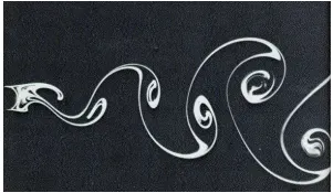
We are taking the flow to be laminar and we are going to change the initial velocity to change the Reynolds number value.
Reynolds number (Re) = `(rho*V*D)/mu`
where
`rho` = density of the fluid (kg/`m^3`)
V = initial velocity of the fluid (m/s)
D = Diameter of the cylinder (m)
`mu` = dynamatic viscosity (kg/`m*s`)
Strouhal Number
The Strouhal number (St) is a dimensionless number describing oscillating flow mechanisms. The Strouhal Number represents a measure of the ratio of the inertial forces due to the unsteadiness of the flow or local acceleration to the inertial forces due to changes in velocity from one point to another in the flow field.
`St = (f*L)/U`
where
`f` = Frequency of vortex shedding (1/s)
L = Characteristic length (In this case Diameter) (m)
U = Flow velocity (`m*s^-1`)
For large Strouhal numbers (order of 1), viscosity dominates fluid flow, resulting in a collective oscillating movement of the fluid "plug". For low Strouhal numbers (order of 10−4 and below), the high-speed, quasi-steady-state portion of the movement dominates the oscillation. Oscillation at intermediate Strouhal numbers is characterized by the buildup and rapidly subsequent shedding of vortices.
Drag Coefficient
The drag coefficient(`C_d`) is a dimensionless quantity that is used to quantify the drag or resistance of an object in a fluid environment. The Drag coefficient is given as:
`C_d = (2*F_d)/(rho*u^2*A)`
where
`F_d` = drag Force (N)
`rho` = density of the fluid (kg/`m^3`)
u = Flow velocity (`m*s^-1`)
A = cross-sectional area (`m^2`)
Lift Coefficient
The lift coefficient (CL) is a dimensionless coefficient that relates the lift generated by a lifting body to the fluid density around the body. It is used to determine the lift of an object in a fluid environment.
`C_L = (2*F_L)/(rho*u^2*A)`
where
`F_L` = drag Force (N)
`rho` = density of the fluid (kg/`m^3`)
u = Flow velocity (`m*s^-1`)
A = cross-sectional area (`m^2`)
Assumption
For the simulation, we have taken the following assumption
`rho` = 1 kg/`m^3`
`mu` = 0.02 kg/`m*s`
Grid element size = 0.025 m
Case Setup
1. First we are going to open the workbench and going to click on the Fluid Flow(Fluent). It is going to open the module in the Project Schematic.
2. Now we are going to click on the geometry. It will take you to the spaceClaim. Now we are going to create the geometry.
Dimensions of the geometry:-
Length of the object = 60 m
Width of the object = 20 m
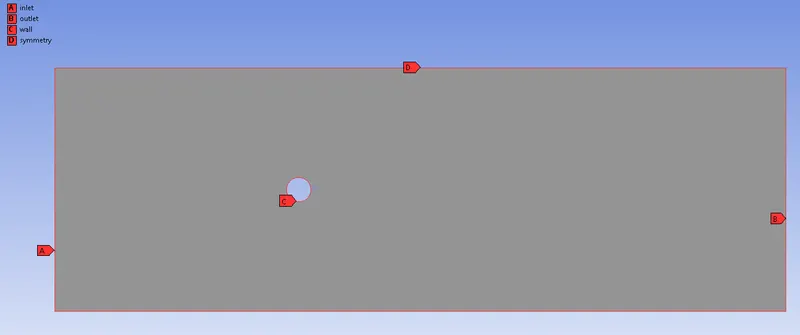
Diameter of the circle = 2 m
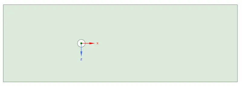
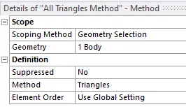
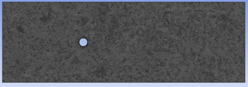
3. Now we are going to open the mesh. It will take us into the meshing. Here we decide what mesh element size we are going to take. I have taken the mesh size to be 0.025 m. We want the mesh to be in the triangle shape. So we are going to click the right button on the mesh and select the inert in which we are going to select method. So we want the surface to be in the triangle shape so we are going to select the surface and we are going to choose the method to be triangle.
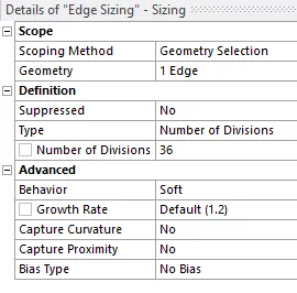
4. Now we are going to change the edge size of the circle so that it could be in a better shape. So we are going to click the right button on the mesh and select the inert in which we are going to select sizing. Now we are resizing circle so we are going to select the circle and in the definition we are going to change the type to be in the number of divisions. We are going to take 36 divisions. It will make the circle to be smooth.
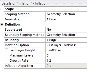
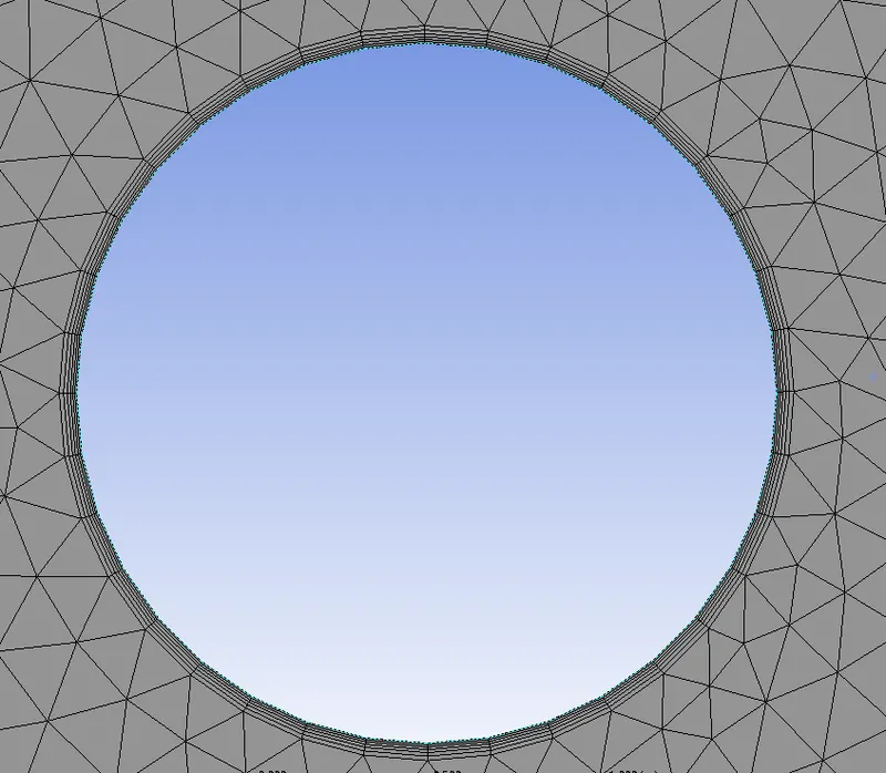
5. The flow around the cylinder is very important so to capture the velocity at the edge properly we are going to use an inflation layer. It makes the mesh to be body fitted. We are going to make the 6 inflation layer with 20% growth rate.
6. Now we are going to give the name to inlet, outlet, wall and symmetry.
Now we are going to generate the mesh and we will get our required mesh.
7. Now we are going to update the mesh. Now we are going to Setup the case. So it will take us to the Fluent. Here we are going to take the model to be laminar flow model.
8. In the Fluent we will go to Physics. Here we choose the type of solver, we have taken the pressure-based type solver. Now we have to choose the velocity formulation, we have taken absolute velocity formulation. Now we are going to choose the time, we are using a steady time and for unsteady case we are going to choose transient.
9. Now we will click on the material. Here we will select the material and give the properties to the material. We are using air with the density 1 kg/`m^3` and viscosity to be 0.02 kg/`m*s`.
10. Now we are going to give the boundary condition. In inlet we are going to give the velocity and at the outlet we are going to give the pressure to be zero (static pressure). Wall to be stationary wall with no-slip condition.
11. We are going to monitor the velocity at a point that is after the cylinder. So we are going to create a point there. I have created the point at the coordinate of (10,0).
12. Now we are going to click on the solution. Here we are going to create the definitions. We want the drag force coefficient, lift coefficient and vertex velocity.
13. Now we are going to initialize the solution and we are going to create the pressure and velocity contour. And we have to change the value in the reference which is present in the result section in reports.
14. Now we are going to simulate the result and we will get the plots and results.
Unsteady State Solver
Case-1
Reynolds number = 100
velocity = 1 m/s
Time step size = 0.1 s
Results
Residual
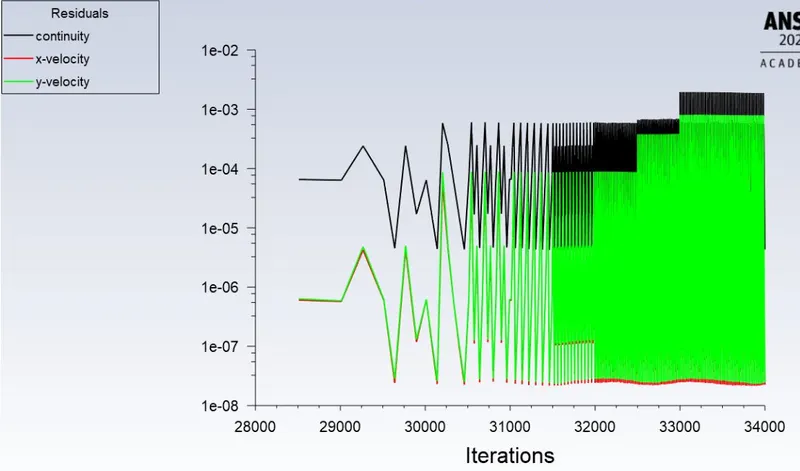
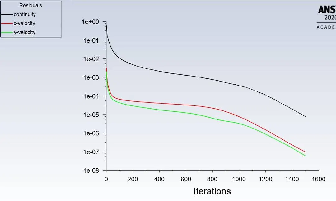
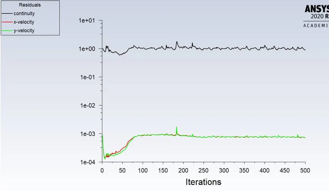
We can see from the graph that after some time it is plotting in the same pattern. So we get converged results.
Vertex Average
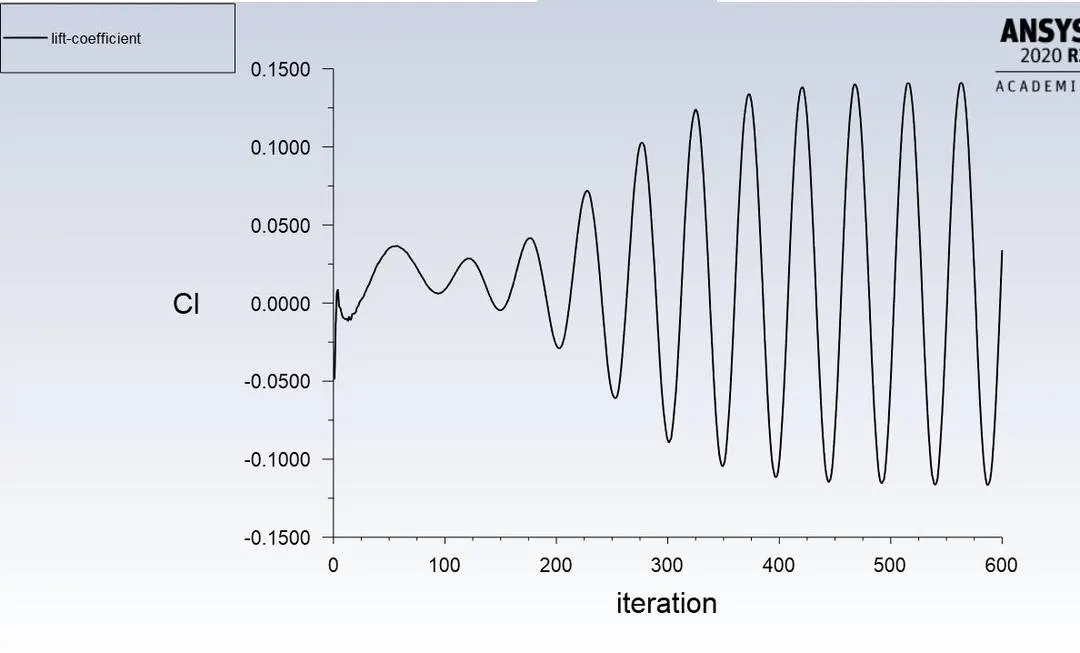
Lift Coefficient
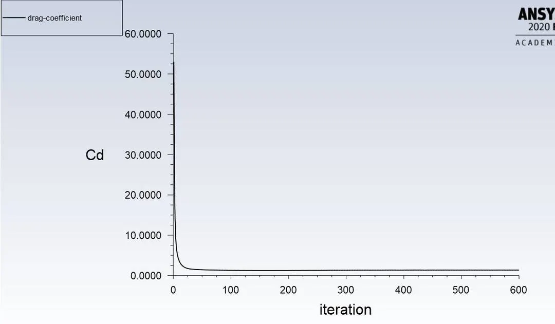
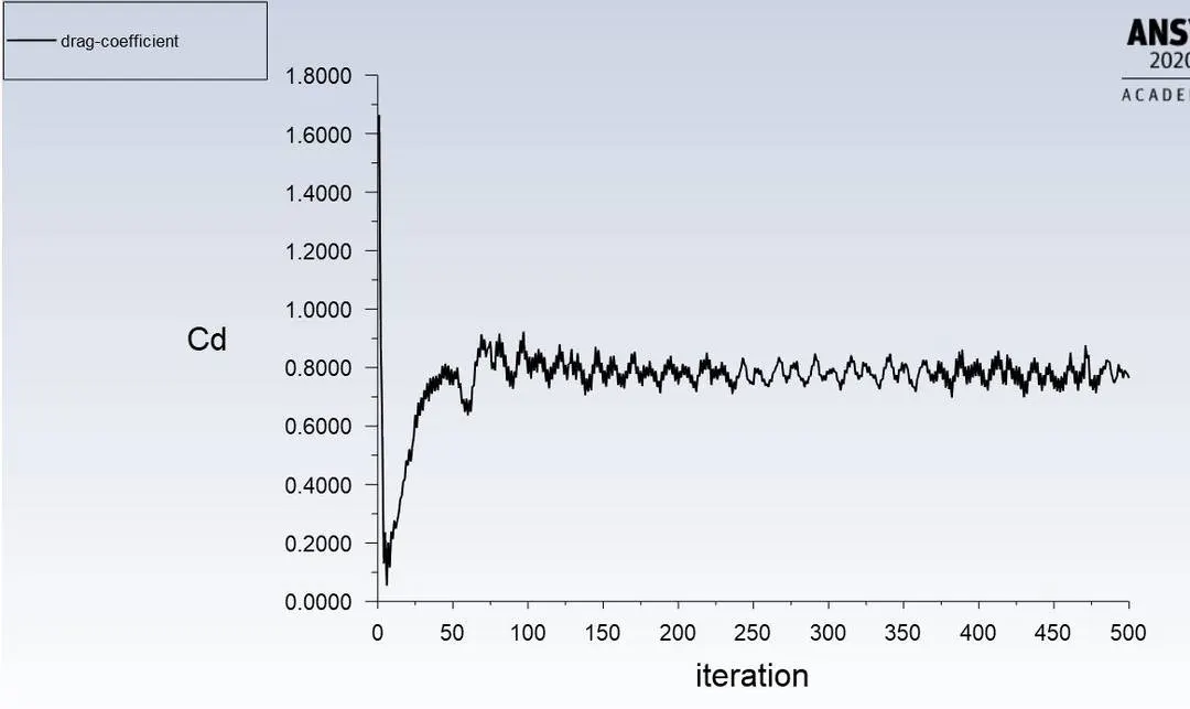
Drag Coefficient
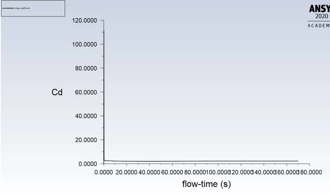
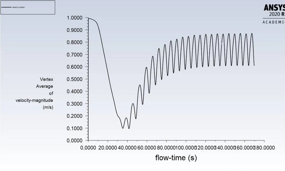
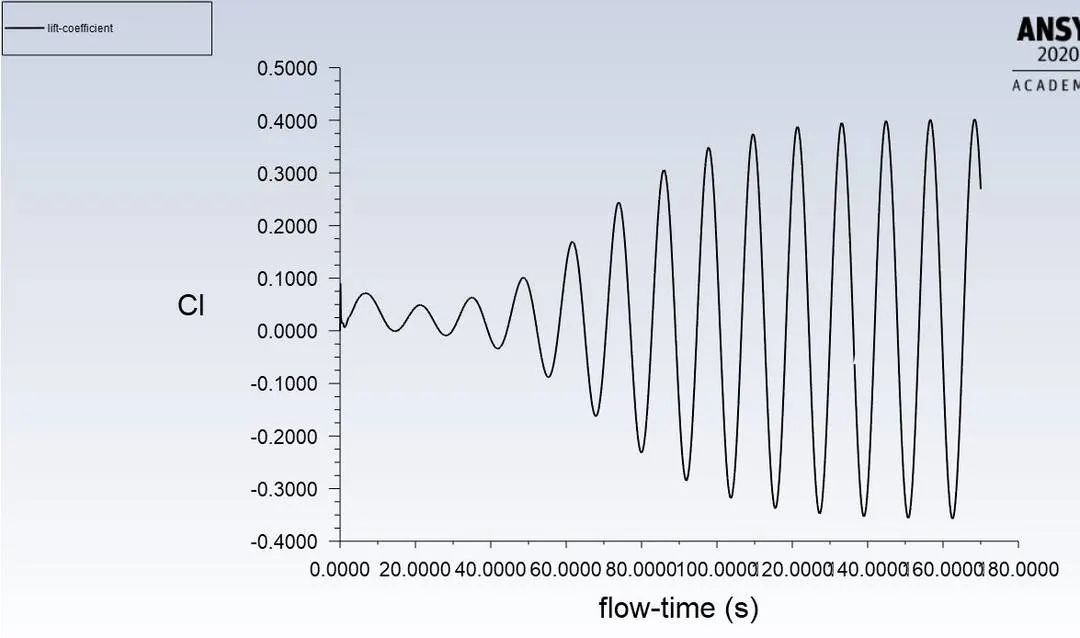
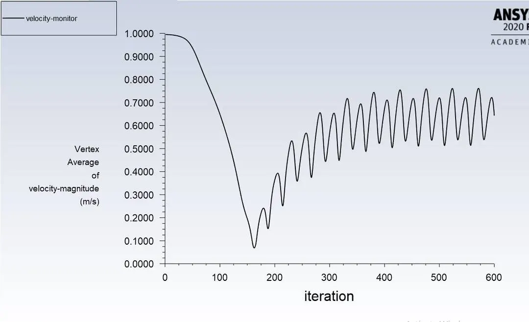
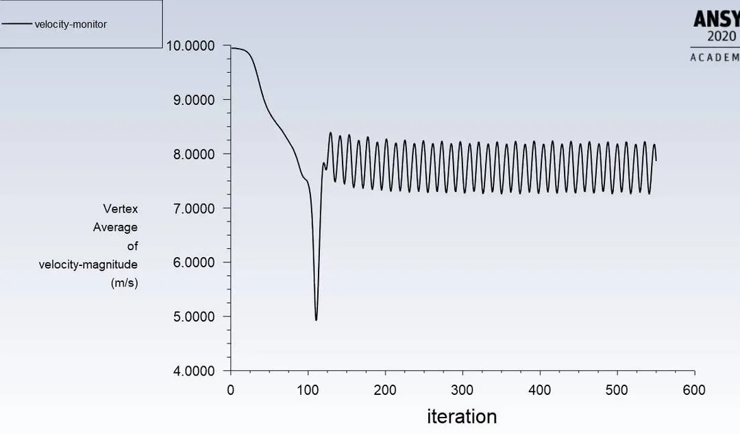
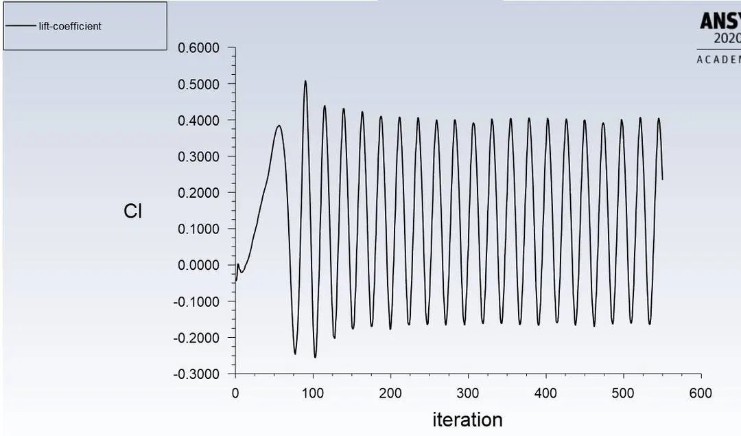
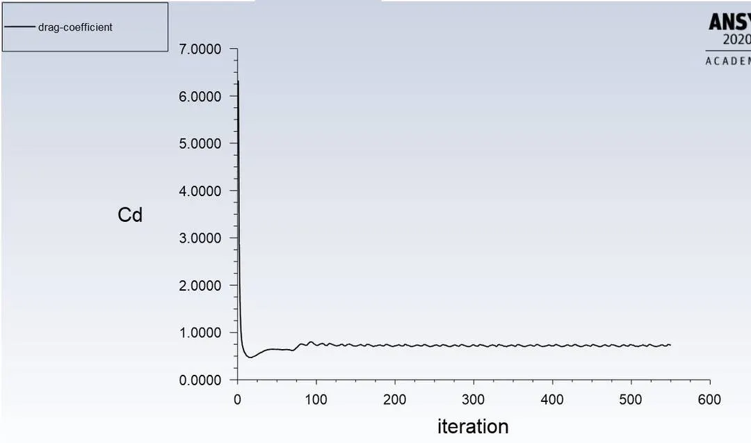
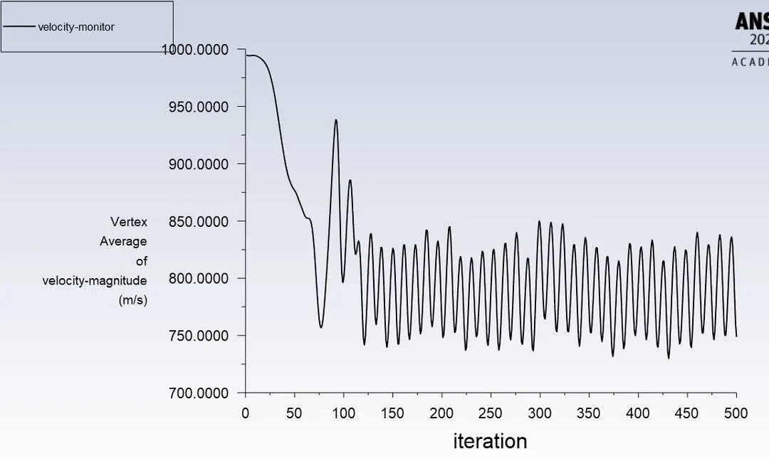
We are getting from the above graphs that the values are repeating in the same pattern or it is constant. So we get the converged results.
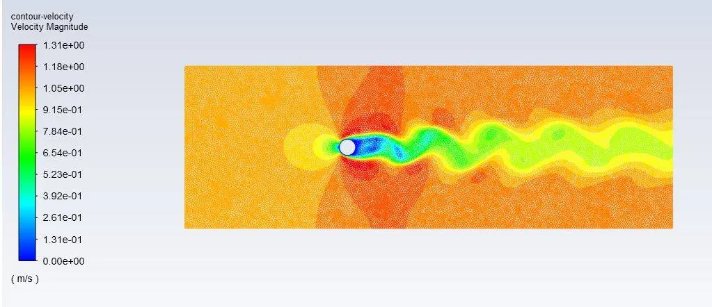
Velocity Contour
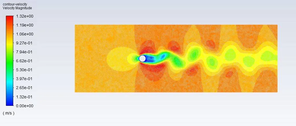
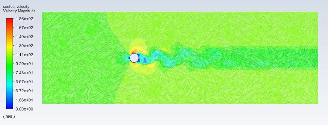
In the velocity contour, we can see that at the end the vortex shedding behind the cylinder should look like the this.
Strouhal Number
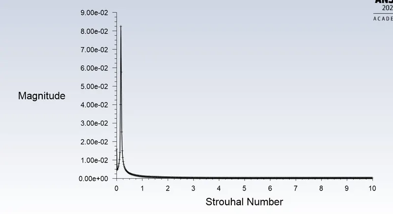
If we check the value of the strouhal number from the data than we will get the Strouhal number numerically to be 0.1634 (data I have uploaded).
Analytical Value
We are going to calculate the strouhal number from the formula
frequency `f = ("Number of cycle")/("Time")`
`f = 1/11.8`= 0.0847 `s^-1`
D = 2 m
U = 1 m/s
So `St = (0.0847*2)/1`= 0.1694
Error
Error = (Analytical value - Numerical Value)/(Analytical Value)
Error = `(0.1694-0.1634)/0.1694` = 3.54%
It is less than the 5%.
Steady State Solver
Case-2
Reynolds number = 100
velocity = 1 m/s
Results
Residual
Vertex Average
Lift Coefficient
Drag Coefficient
Velocity Contour
Inference
We can see from these two cases that we get the converged values faster in the steady-state solver.
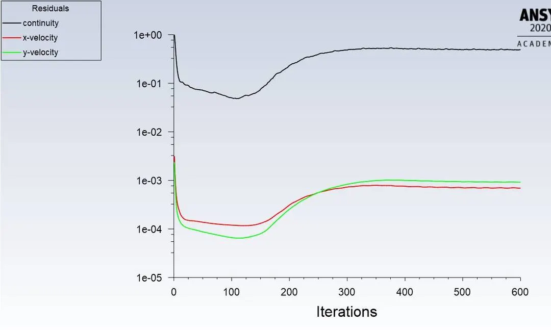
We can see from the plots that after some time the values does not changes or they start to repeat the same pattern so we can say that from the above graphs that we get the converged results.
Steady State Solver
Case-3
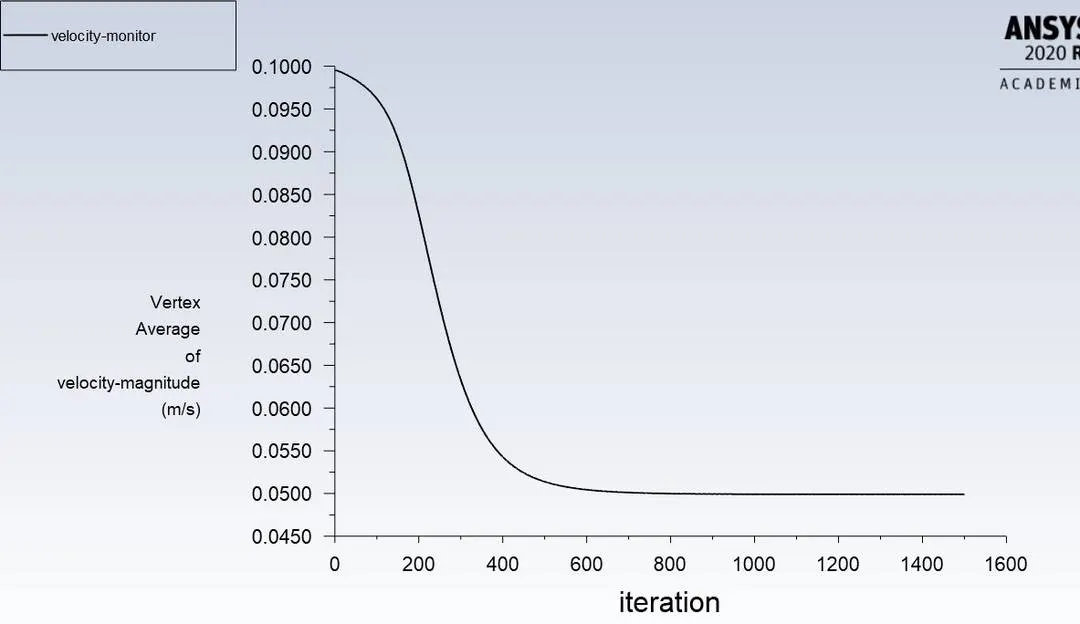
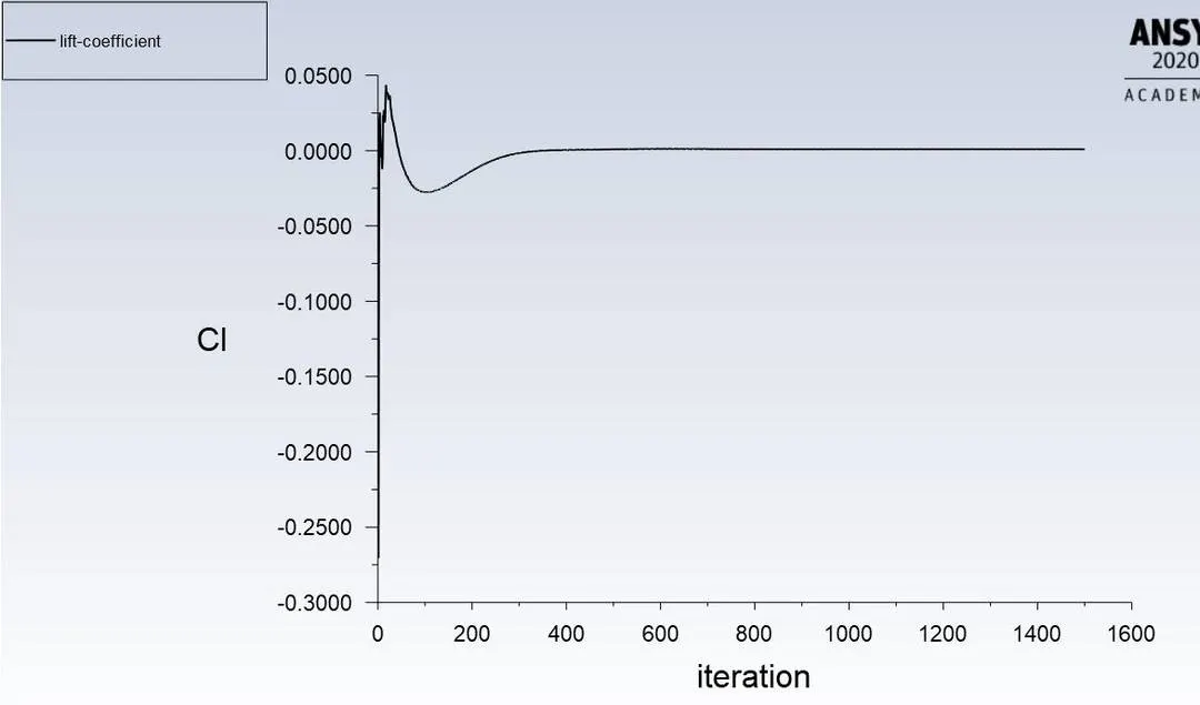
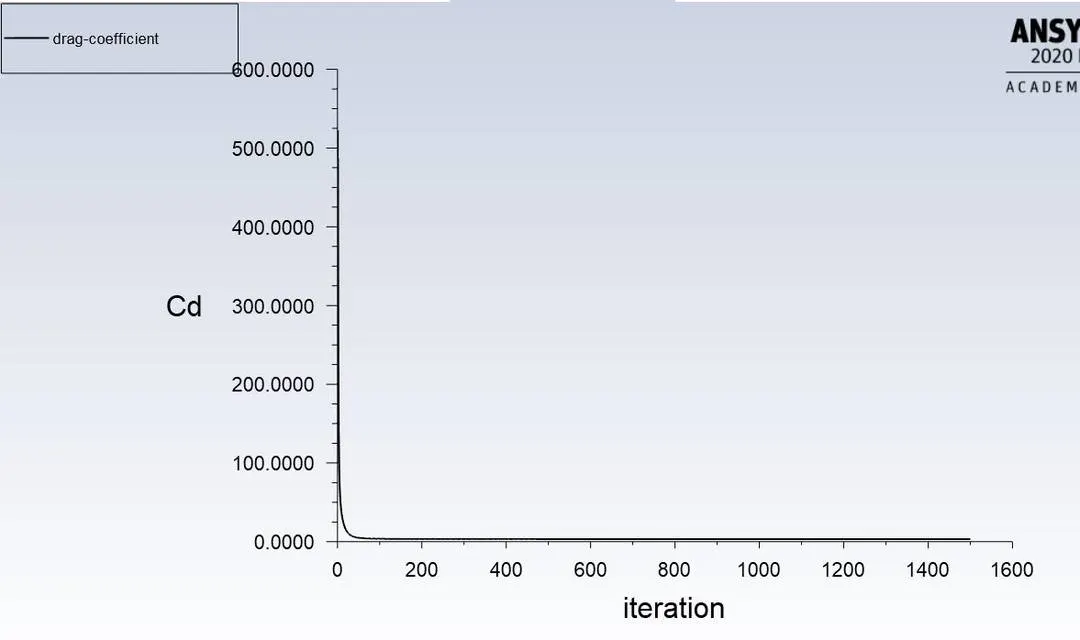
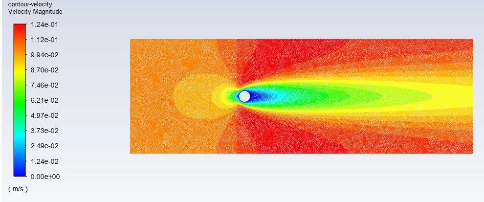
Reynolds number = 10
velocity = 0.1 m/s
Results
Residual
Vertex Average
Lift Coefficient
Drag Coefficient
Velocity Contour
Steady State Solver
Case-4
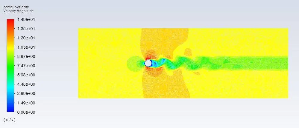
Reynolds number = 1000
velocity = 10 m/s
Results
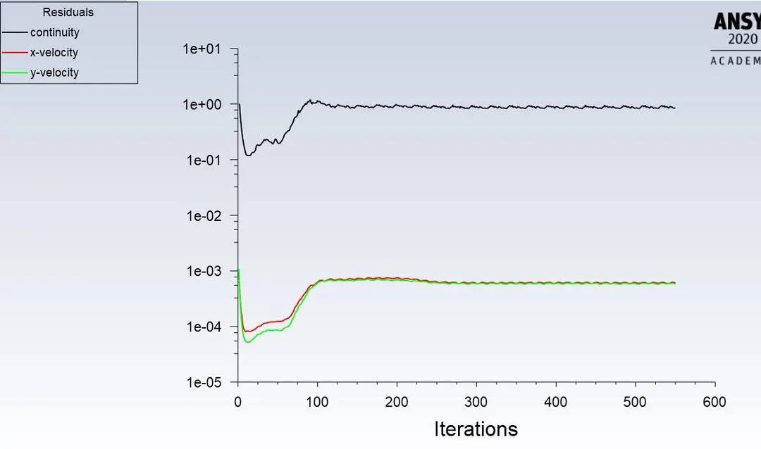
Residual
Vertex Average
Lift Coefficient
Drag Coefficient
Velocity Contour
Steady State Solver
Case-5
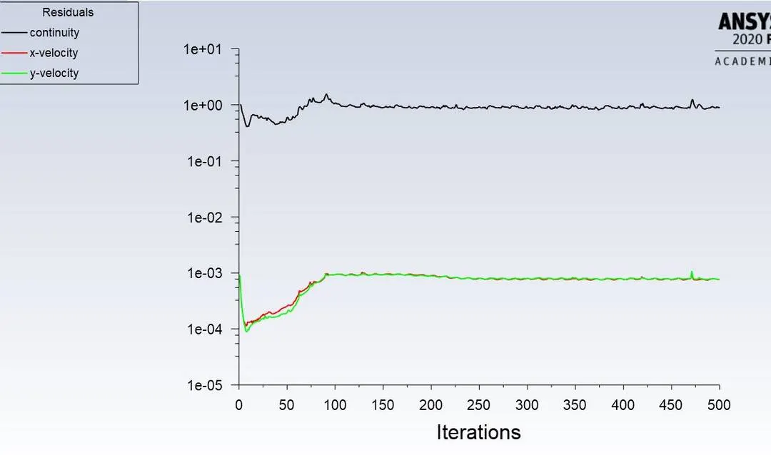
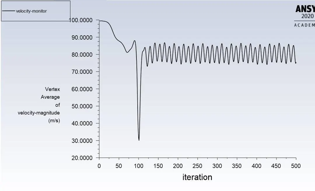
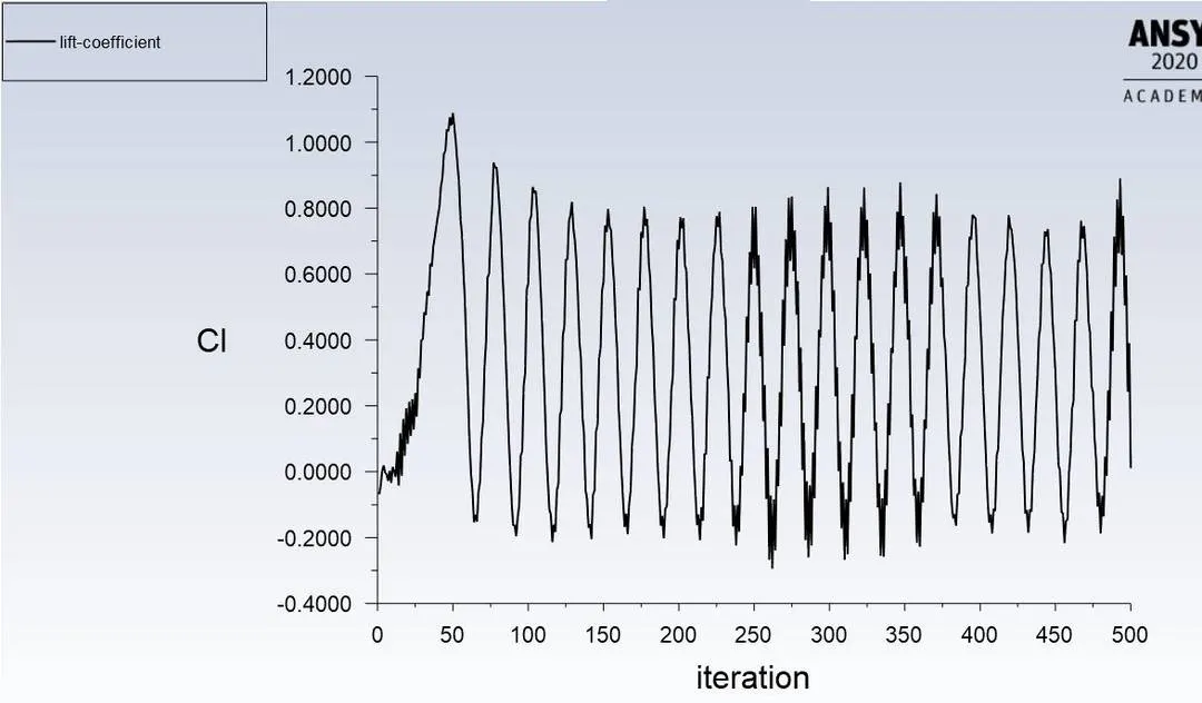
Reynolds number = 10000
velocity = 100 m/s
Results
Residual
Vertex Average
Lift Coefficient
Drag Coefficient
Velocity Contour
Steady State Solver
Case-2
Reynolds number = 100000
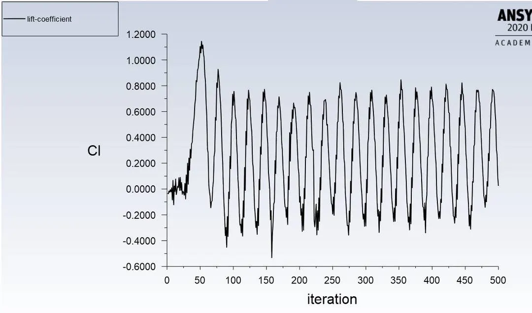
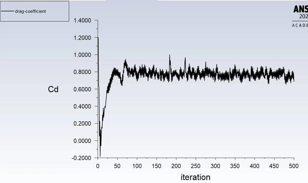
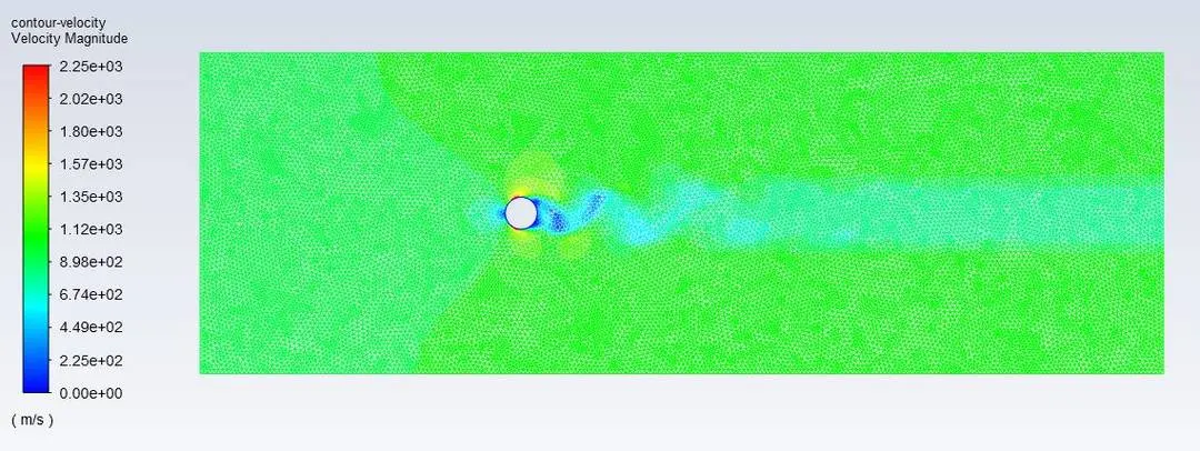
velocity = 1000 m/s
Results
Residual
Vertex Average
Lift Coefficient
Drag Coefficient
Velocity Contour
Comparision
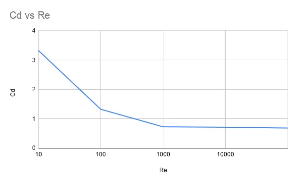
| Velocity (m/s) | Reynold Numbers(Re) | Drag Coefficient(`C_d`) |
| 0.1 | 10 | 3.3241 |
| 1 | 100 | 1.3248 |
| 10 | 1000 | 0.7281 |
| 100 | 10000 | 0.7138 |
| 1000 | 100000 | 0.6862 |
The chart between Drag force Coefficient and Reynold Number
Conclusion
So from the above comparison, we can get the following conclusion:-
1. We are taking the reference paper as our validation. So first we simulate the values for the Reynold number 100 and compare the drag coefficient with the reference paper value. We are getting the values almost the same (the error is less than 5%).
Numerical value I get = 1.3248
Referece value = 1.3353
error = 0.786%
So we are going to use this method for the other simulation.
2. When we increase the Reynold numbers drag coefficient values decreases.
3. We can see that at Reynolds number we didn't get the vortex, we get the vortex when we take the Reynolds number to be 100. In the beginning we say that to get the vortex shedding Reynold number should be at least 48 (From the research paper).
4. When we increase the Reynold number, residual values also increase. Because of the velocity oscillations, it increases.