Steady Vs Unsteady flow over a cylinder
AIM: The aim of the challenge is to simulate flow over a cylinder and to explain the phenomenon of Karman vortex street.
Karman Vortex Street: In fluid dynamics, a Kármán vortex street (or a von Kármán vortex street) is a repeating pattern of swirling vortices, caused by a process known as vortex shedding, which is responsible for the unsteady sepration of flow of a fluid around blunt bodies.
Vortex shedding: In fluid dynamics, vortex shedding is an oscillating flow that takes place when a fluid such as air or water flows past a bluff (as opposed to streamlined) body at certain velocities, depending on the size and shape of the body. In this flow, vortices are created at the back of the body and detach periodically from either side of the body forming a von Kármán vortex street.
Strouhal number:
In dimensional analysis, the Strouhal number is a dimensionless number describing oscillating flow mechanisms.
The Strouhal number is given as

where f is the frequency of vortex shedding, L is the characteristic length and U is the flow velocity. In certain cases, like heaving (plunging) flight, this characteristic length is the amplitude of oscillation.
Geometry:
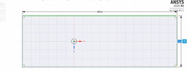
We first prepare our geometry to do so we prepare our geometry using spaceclaim in Ansys fluent.Below is the generated geometry with cylinder of diameter 2 m.
Meshing:
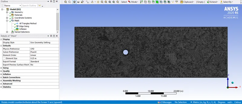
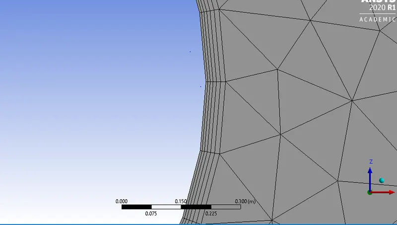
The meshing of the geometry is done using triangular mesh, initially when mesh is loaded we can see the baseline mesh.The triangular mesh method is applied to the given geometry for meshing.Mesh of size 0.25m is applied for finer mesh.Here we have employed the edge sizing for the circular cylinder area of the geometry. this is done to refine the shape of the geometry as traiangular meshing results into irregular surface of the cylinder we have taken 36 number of divisions considering one division for each 10 degrees of circular shape.further, as we need to capture flow around the cylinder we use inflation layers around the cylinder. we have applied 6 layers of inflation with 0.005m of thickness layer and also an increment of 1.2 for each layer. this method is called body fitted mesh as we generate the layers to fit around the shape of geometry. we then update the mesh and also name the geometry as inlet outlet walls and symmetry.
Geometry meshing:
Body fitted meshing showing inflation layer around the cylinder:
SETUP:
1)Setting up physics: We have used pressure based steady state/transient state solver with laminar model.we have seleted user defined material with density= 1kg/m3 and viscosity=0.02kg/m-s. boundary consitions: inlet velocity=1m/s and outlet pressure = 1 atm
2)Solution defination: setup a monitor point at a distance of 4*d(diameter) from the center of cylinder using the create surface tool in results section. the monitor point is setup in order to capture the vertex average of velocity magnitude.further we also setup the plot for drag and lift coefficient.
3)intialize the solution using hybrid methos for steady state solution and standard solution for transient solution to setup the pressure and velocity contours in the result section in order to visulaize the pressure and veocity changes.
part1)
Steady state with Reynolds number 100
Hybrid initialization is done with number of iteration=1000.
Residual Plot:
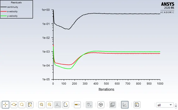
The residual plot shows that the solution is converged as plot is showing staright line after 400 to 500 iterations.
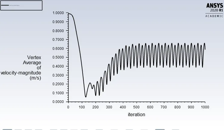
Vertex average of velocity magnitude:
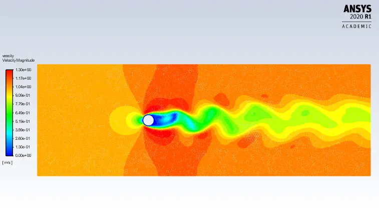
Velocity Contour:
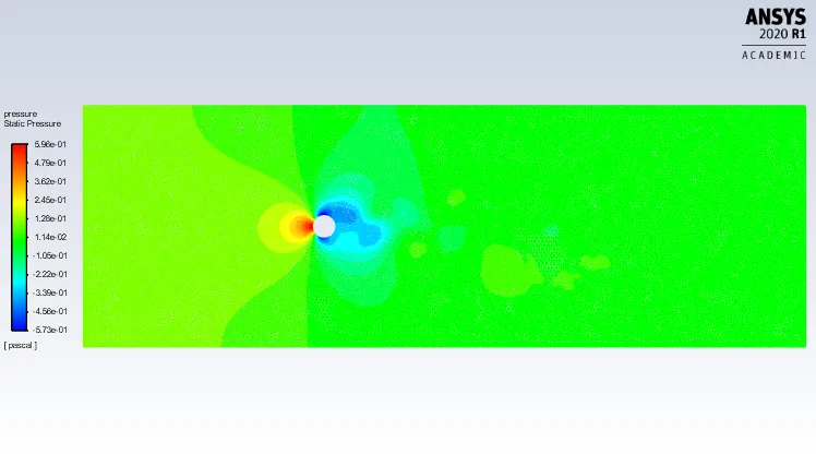
Pressure Contour:
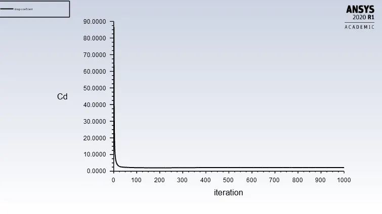
Drag Coeffcient:
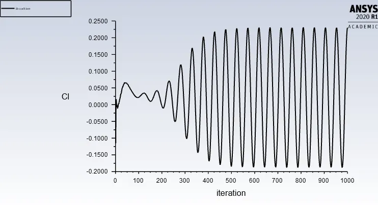
Lift Coeffcient:
Strouhal number:
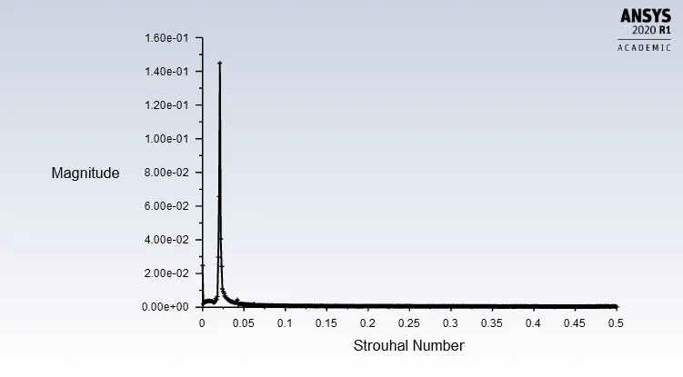
The above plot is plotted using the FFT by spectral analysis of lift coeffcient to setup the plot we have taken strouhal number on x axis function and magnitude on y axis function.
The strouhal number for staedy state case with Re=100 is 0.14.
Animation showing vortex shedding for staedy state case with Re=100.
Transient state solution:
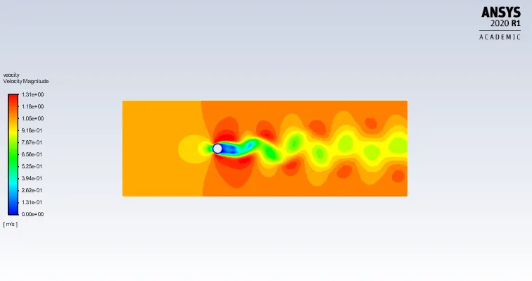
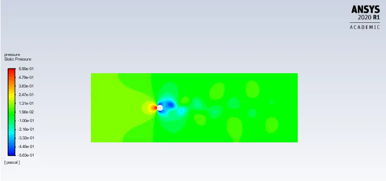
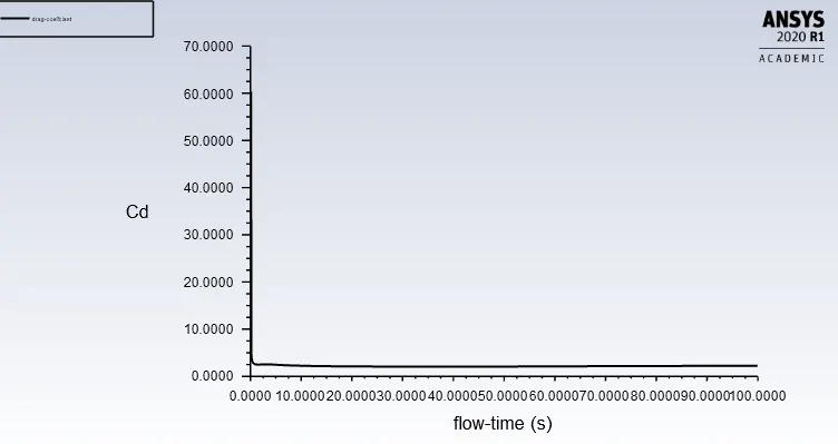
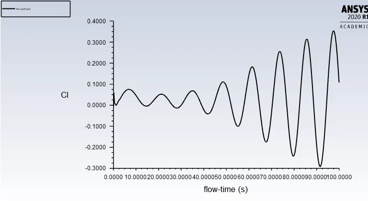
In case of transient state solver we employed standard initialization method with time steps of 1000 and step size of 0.1 sec.
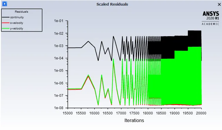
Residual Plot:
The plot shows the oscillation of residual values above 18500 iterations which is the sign that the simulation has converged.
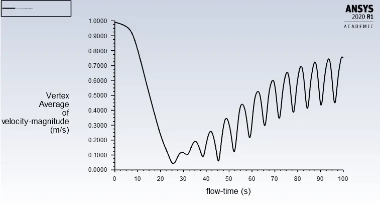
Vertex average of velocity magnitude:
The vertex avg velocity magnitude plot also shows oscillation that are repaeating as similar maximum and minimum peak points repeatedly that also confirms that the results have converged.
Velocity Contour:
Pressure Contour:
Drag Coeffcient:
Lift Coeffcient:
Strouhal number:
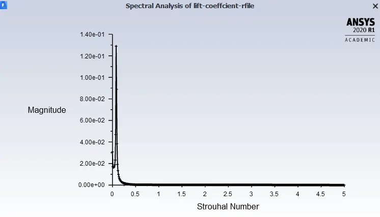
The above plot is plotted using the FFT by spectral analysis of lift coeffcient to setup the plot we have taken strouhal number on x axis function and magnitude on y axis function.
The strouhal number for transient state case with Re=100 is 0.13.
Animation showing vortex shedding for Transient state case with Re=100.
Part 2)
For part 2 of the challenge we are supposed to Calculate the coefficient of drag and lift over a cylinder by setting the Reynolds number to 10,100,1000,10000 & 100000 and discuss the effect of Reynolds number on the coefficient of drag. For this purpose we have set reynolds number by varying the velocity and keeping the viscosity (0.02kg/m-s) and density (1 kg/m3) as constant.
Reynolds no=10:
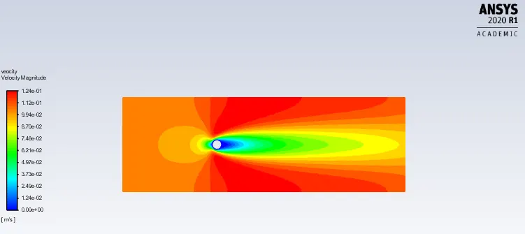
Re=10, density=1 kg/m3,viscosity=0.02kg/m-s, velocity=0.1,daimeter of cylinder=2m,
Drag coefficient plot:
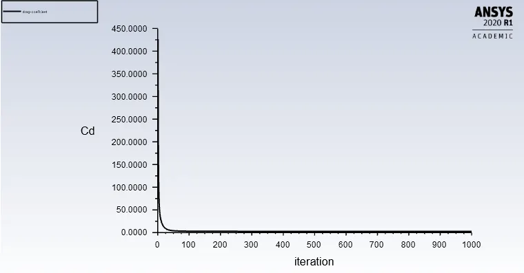
Drag Coeffcient=Cd=2.7136
Lift Coefficient plot:
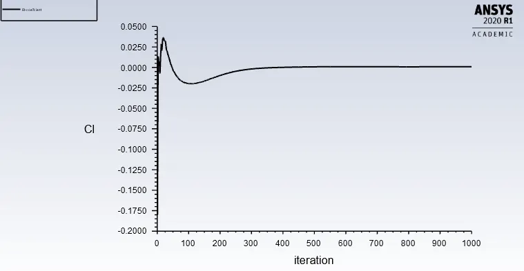
Lift Coeffcient=Cl=0.0007580
Velocity Magnitude plot:
Reynolds no=100:
Re=100, density=1 kg/m3,viscosity=0.02kg/m-s, velocity=1,daimeter of cylinder=2m
Drag coefficient plot:
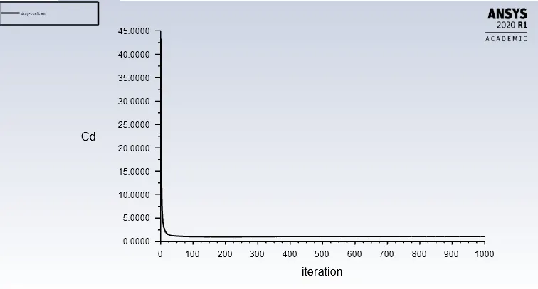
Drag Coeffcient=Cd=1.09379
Lift Coefficient plot:
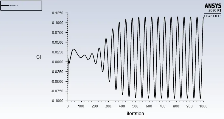
Lift Coeffcient=Cl=0.11490
Velocity Magnitude plot:
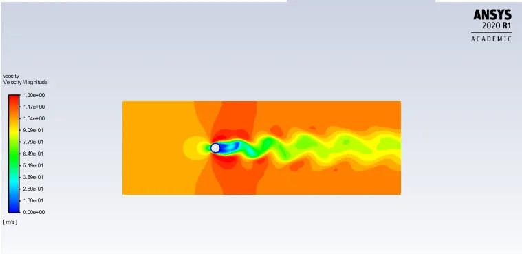
Reynolds no=1000:
Re=1000, density=1 kg/m3,viscosity=0.02kg/m-s, velocity=10,daimeter of cylinder=2m
Drag coefficient plot:
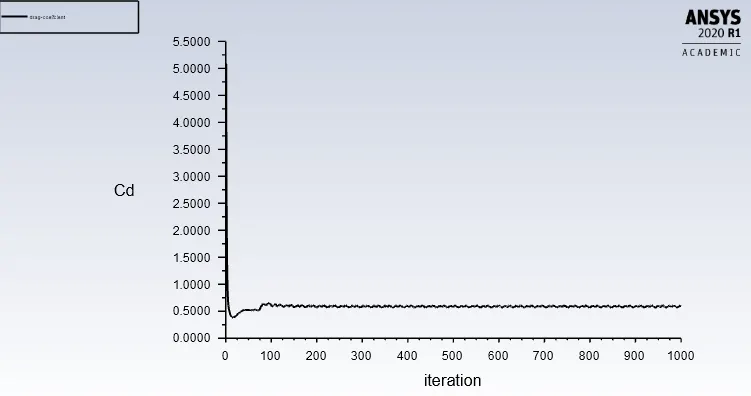
Drag Coeffcient=Cd=0.5890
Lift Coefficient plot:
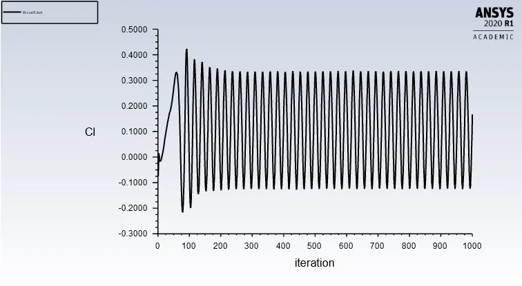
Lift Coeffcient=Cl=0.16667
Velocity Magnitude plot:
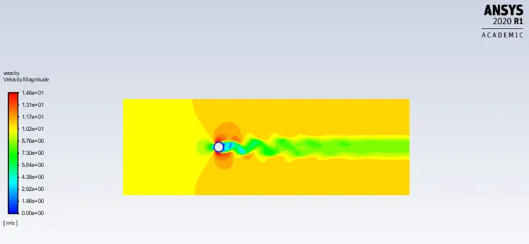
Reynolds no=10000:
Re=10, density=1 kg/m3,viscosity=0.02kg/m-s, velocity=100,daimeter of cylinder=2m
Drag coefficient plot:
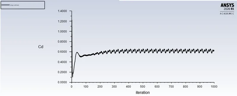
Drag Coeffcient=Cd=0.64879804
Lift Coefficient plot:
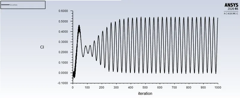
Lift Coeffcient=Cl=0.54258696
Velocity Magnitude plot:
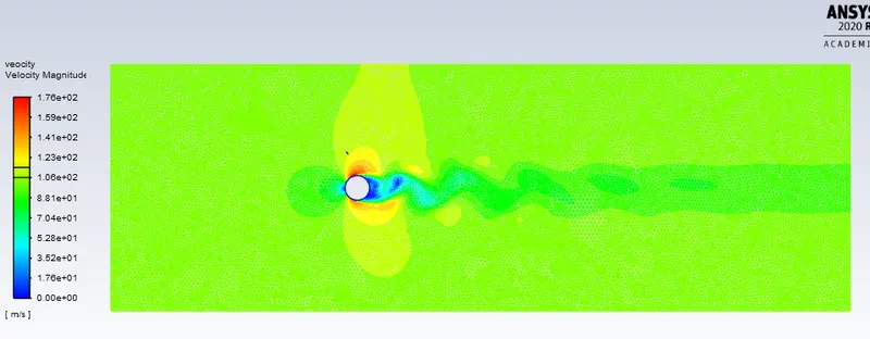
Reynolds no=100000:
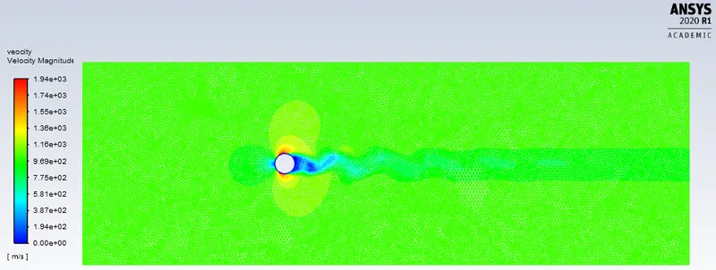
Re=10, density=1 kg/m3,viscosity=0.02kg/m-s, velocity=1000,daimeter of cylinder=2m
Drag coefficient plot:
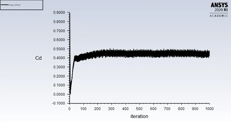
Drag Coeffcient=Cd= 0.40285365
Lift Coefficient plot:
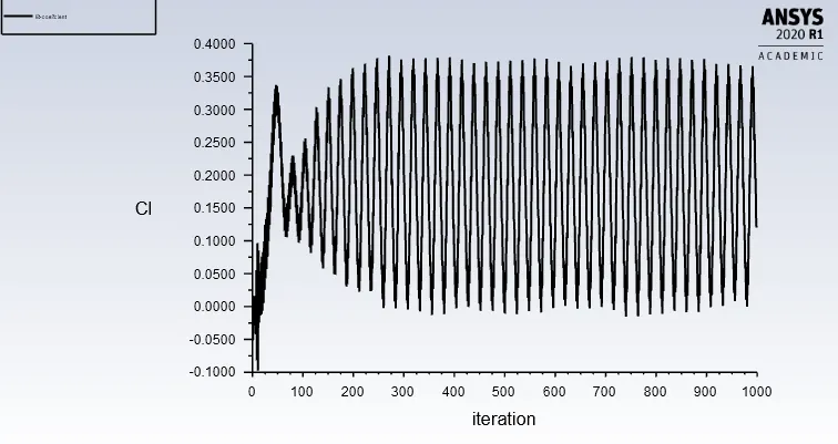
Lift Coeffcient=Cl=0.053811072
Velocity Magnitude plot:
Results:
|
Sr.No |
Reynolds Number |
Drag Coeffcient Cd |
Lift Coeffcient Cl |
|
1 |
10 |
2.7136 |
0.0007580 |
|
2 |
100 |
1.0979 |
0.1149 |
|
3 |
1000 |
0.5890 |
0.1667 |
|
4 |
10000 |
0.64879 |
0.54258 |
|
5 |
100000 |
0.40285 |
0.05381 |
Conclusion:
1)The Staedy state analysis of flow over cylinder with varying range of reynolds number shows that when reynolds number is increased the drag coeffcient goes on decreasesing.There are really 2 contributions to the drag force. One comes from the inertia of the fluid (the object actually collides with molecules) and the other comes from the viscosity. As Re increases, the size of the viscosity, relative to the other parameters, is decreasing. This means that the viscosity term in Navier-Stokes equation is relatively less important. Since the viscosity plays a smaller role, we would expect the contribution to drag due to viscosity to decrease.
2)The large dive in the drag coefficient is called the drag crisis. This happens when the boundary layer over the cylinder transitions from laminar to turbulent. Turbulent boundary layers are more resistant to separation, so the flow stays attached longer resulting in decreased form drag.
3)We can see the drag coefficient rises again as more and more of the cylinder has a turbulent boundary layer. at higher reynolds number. Turbulent boundary layers have a higher skin friction coefficient than their laminar counterparts.The plot goes to higher Reynolds numbers the drag coefficient would level off and then eventually probably decline again.
4) The lift coeffcient goes on increasing as the reynolds number increases. in laminar regime the lift coeffcient is very low as drag is on higher side.
5) For reynolds number above 2000 the flow becomes turbulent hence i have applied k-omega sst model for Re=10000 and 100000. At reynolds number 10 we cannot see vortex shedding in velocity plot.A very interesting sequence of events begins to develop when the Reynolds number is increased beyond 40, at which point the wake behind the cylinder becomes unstable. The wake develops a slow oscillation in which the velocity is periodic in time and downstream distance. The amplitude of the oscillation increases downstream. The oscillating wake rolls up into two staggered rows of vortices with opposite sense of rotation.
Reference material:
https://www.sciencedirect.com/science/article/pii/S0307904X08000243