State Space Trajectory of Neurons using PCA (Python implementation)

Background:

PCA - Principal Component Analysis.

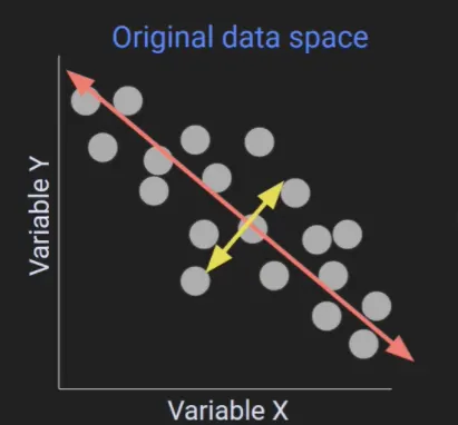
Fig: plotting 2 variables on the same plot from a dataset

Imagine we have a 2 variable dataset. Clearly there is some correlation between the variables, some sort of relationship between them.

PCA will identify the axis of maximal similarity or maximal covariance of the 2 variables x and y. Then it will rotate/reorient the data space so that the axis of maximum correlation becomes principal component 1 and the other the principal component 2 . Both are orthogonal to each other.

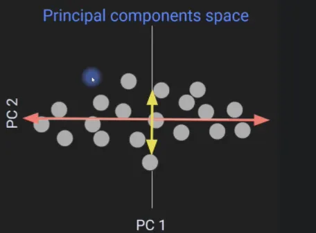
Fig: Same data above drawn using the Principal component axis

This allows us to redraw the data in "Principal component space."

Like so,

Same data, just rotated. Imagine that the PC1 dimension is important/relevant but PC2 is just noise/not relevant/important

So we want to ignore PC2 and use PC1.

That's one of the things we do with PCA , compress the data, Dimension reduction

Now same data points but just one dimension, lost PC2

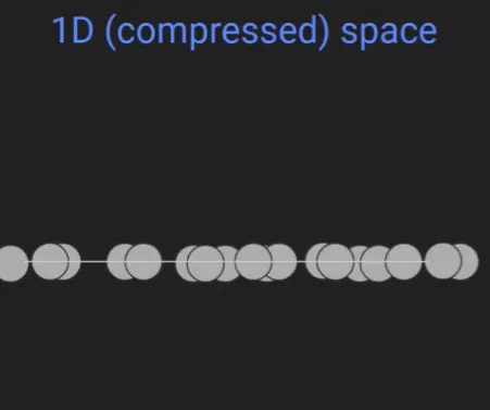
Fig: same data points but now in just one dimension(Principal component 1 )

Inpractice there are many dimensions.

in the project

We will work with 64 dimensional space and compress it down to 2 dimensions.

Then the data in theory will also contain dimensions 3 through 64 but we will be ignoring those.

Tuning : preferences of Brain cells

Motor homunculus that there is a spatial representation of information in your body that is represented in your brain.

Fig: motor Humunculus (to depict that particular neurons related to a particular movement/activity/stimulus are spacially present in different part of the brain )

Example:

We could stick an electrode say in that part of the brain where we see that thumb. Then we will find a brain cell that becomes very active when you move a thumb but does not become active when you , say , blink your eyes, it does not respond, that neuron does not care. That is it only reacts to the stimuli of moving the thumb.

So we can say that brain cell is ‘tuned’ for the muscle movement in th thumb.

Another example, in visual cortex of brain V1

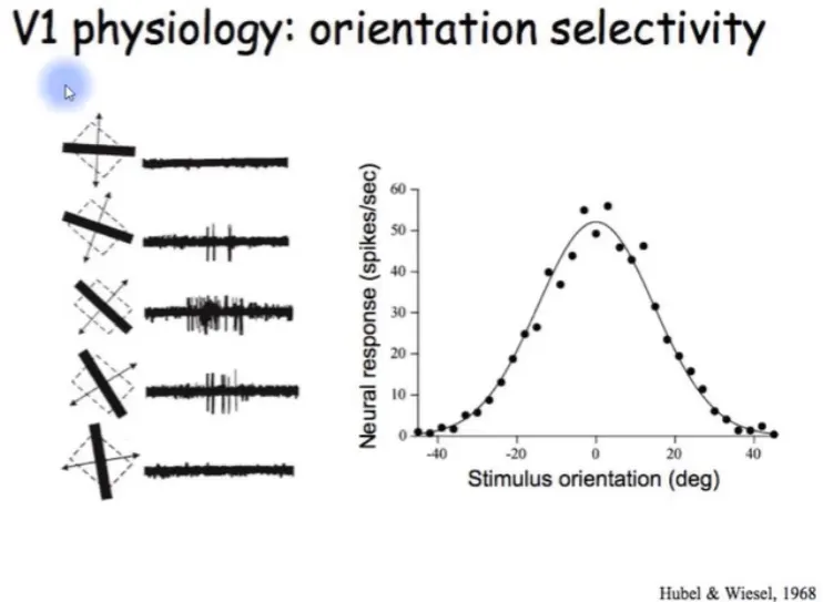
Fig: response from a neuron in the visual cortex V1 region to a rotating beam of light

We see activity of a single brain cell, it becomes really active when a bar of light in front of the subject and in a particular orientation. Exactly same brain cell cares about a particular stimuli, here a particular orientation of light.

The project

Data we will work with:

Fig: the published paper ( our data source )

Data will be from this publication data set. it will not be the whole data set but a part of it.

How data was recorded?

What the scientist did was record individual neurons from the mouse brain . In the experiment the mouse was sometimes licking to the right , sticking its tongue to the right while sometimes it did that to the left

The neurons from where they recorded the data

Then they found the brain cells that become very active when the mouse licked to the right and when it licked to the left.

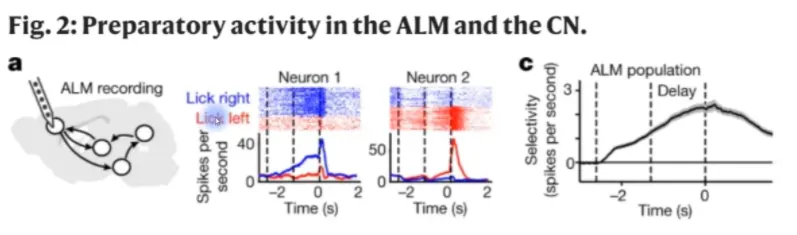
Fig: 2 Neuron's activity. One tuned for the left licking and other for the Right licking of the tongue

So in the figure we see the neuron 1 which became very active when it licked to the right and not very active when it licked to the left.

Neuron 2 became very active when it licked to the left and not very active when it licked to the right.

So neuron1 was tuned for right lick and neuron 2 was tuned for left lick.

Time = 0 is when the lick actually happened, the lick happens at t=0.

the activity plotted

The blurrish blue and red in the activity is actually a row of dots it is a blue dot or red dot if neuron is active and a white dot if it is not active. each row of dots is actually a repitition of the experiment/ trials

So we see a lot of blue dots in the right lick for neuron 1 showing a lot of activity in neuron 1 since it is 'tuned' for the right lick but very few red dots as neuron1 is not tuned for the left lick, so more whitish .

Then it is the solid lines is the average of all the blue trials(right lick i) and red trails (left lick ).

So neuron 1 is tuned for right lick, it has a ‘preference’(terminology) and neuron 2 is tuned for left lick.

The Project:

• Small data from the paper . Visualize the data
• Clean it
• See what the activity looks like
• It has 64 channels(64 neurons)
• Then we will do a PCA to see whether there is some dynamic occurring in a lower dimensional feature space that we can extract by looking at the correlational structure across the 64 neurons.

so in our data the signals coming will be from 64 neurons out of which the neurons which are 'tuned' for the left lick and the right lick will be present.

in these 64 neurons some will be tuned for the right lick while the others will be tuned for the left lick, but the behavior of the same type tuned neurons will be same. That is , those neurons which are tuned for the right lick(the preffered side) will have activity that will be significant because of that stimuli. There will also be other activity too but that will be negligible in size compared to the activity due to the stimuli and also a part of it will also be introducted due to the noise from the measurement apparatus and other artifacts.

so the most important / significant 'features' will be that of the licks while the other will be considered as nonsignificant or not of interest. So we will take the 2 most significant features , in both the cases ,the preffered lick and the the non-preferred side lick.

therefore we will do the analysis to get these 2 most significant/ of interest Principal components. So we will find only the first 2 Principal components in both the Preferred and Non-Preferred data.

Part I : importing , inspecting and cleaning the data
data is in the form of MATLAB .mat file import from disk or drive

we have 2 data matrices

1. one if the preferred licking direction (tuned)
2. one of them is the non-preferred direction (non-tuned)

we can import data in 2 ways: one is to directly upload the file from the device we are are working on and the other is to mount the Google Drive onto the Goggle Colab(note that this is possible when using the goggle colab IDE only)

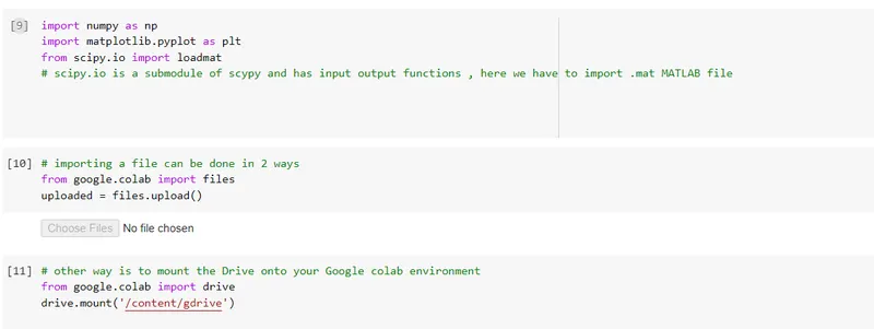
Fig: imported the required libraries and cells for both ways to import the file we have to work with

libraries needed: numpy - for numerical analysis

matplotlib.plyplot - for plotting the graphs and figures

scipy.io - for importing the .mat file that contains the signals information

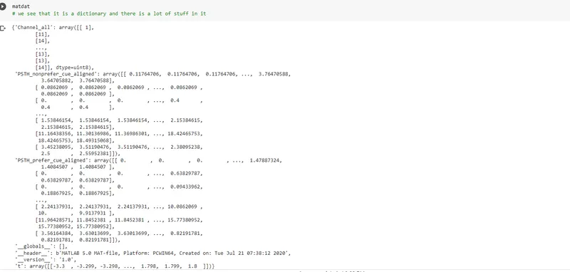
Fig: looking at the content of matdat(the .mat file)

we see it is a dictionary with keys as following:

1. Channel_all : rows of the data matrix, each row corresponds to a particulat channel/neuron trial
2. PSTH_nonprefer_cue_aligned: non-preferred acitvity data matrix
3. PSTH_prefer_cue_aligned: preferred acitvity data matrix
4. t: time vector

so to work with them easily and reduce the variable name size we assign each to a new variable :

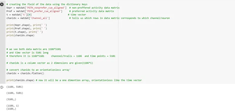
Fig: Nopr,Pref,t, chanidx as the new variables and looking at the sizes of each we see

data matrices are: 1186*5101 for the Preffered and Non-Preffered data matrix

and the Chanidx has 1186 valuesand the time vector has 5101 values

which means we have 64*trials=1186 channel traials with each trial having 5101 time points recorded.

Visualizing the Data matrix we imported:

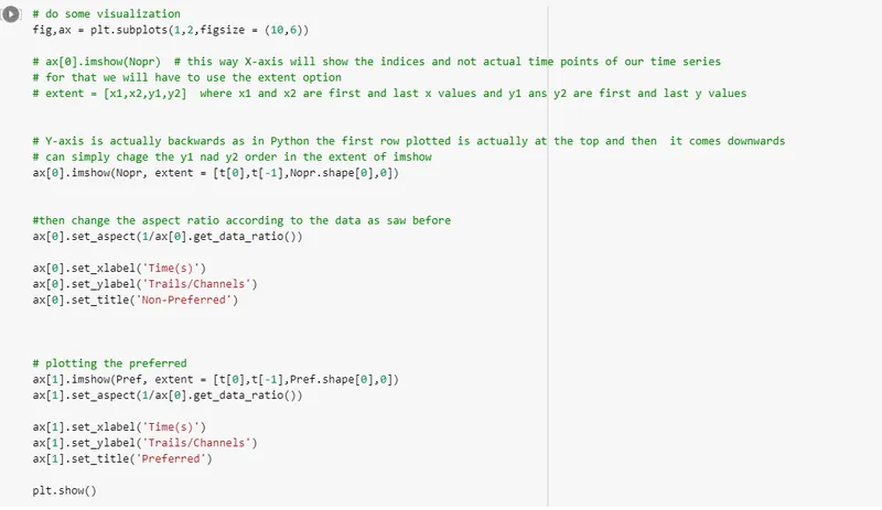
Fig: code to visualize the 2 data matrices

we see the following matrices

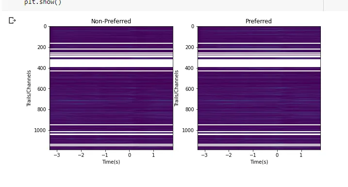
Fig: images of the imported Data matrices (Preffered Movement and Non-Preferred movement)

we see: it has certain white lines which we will discover later that it has no data at all and part of cleaning the data is the removal of these artifacts introduced in the data matrix.

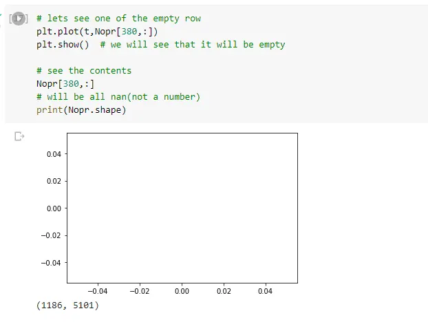
By visual inspection: it seems that the 380th row does not have any data, so we try to plot its time series and we observe nothing is plotted so it can be said that these rows are to be removed as they do not hav any data at all.

Looking at the Data Another way: plotting each trial timeseries as a line

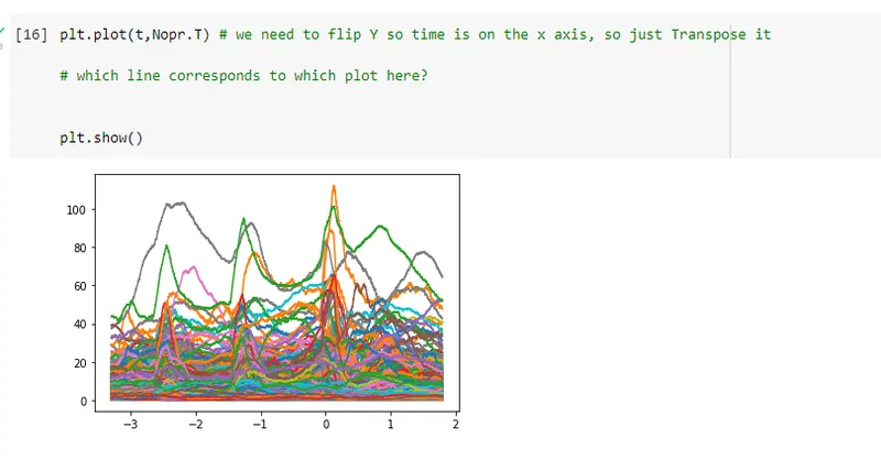
Fig: plotted each trial as a line so it has 1186 lines (including the empty artifacts)

we see that we had only 64 neurons/channels but here the chanidx contains 1186 rows? To further investigate we will see the actual values of the chanidx. to see the unique values in chanidx.

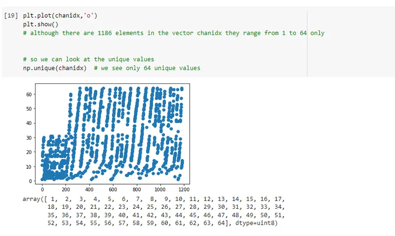
Fig: we first plot and see that all the dots are limited within the y=64 and y=1

looking at the unique values in the vector we see it only has values of 1 to 64

this means that the same neuron has been taken for trials multiple times

where the value of the chanidx element represents the Neuron and the row contains the time series of the particular trial recorded from that particular neuron.

cleaning the data

because we saw those empty timeseries artifacts we have to remove them to clean the data.

will use the isfinite() function

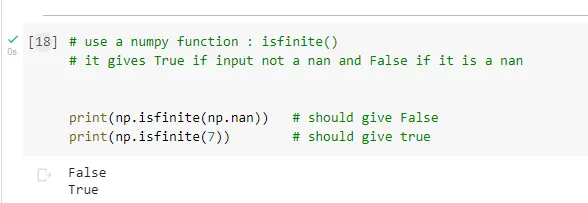
Fig: working of the isfinite() function . Retursns true if finite and False if not (nan - not a number)

Applying this to our data set, we will check the first element of all rows and get a vector of True and False and then input them inside our data matrix. This will eliminate all the rows that are non-finite completely. This will keep the rows whose first element is finite and the rest will be dropped.

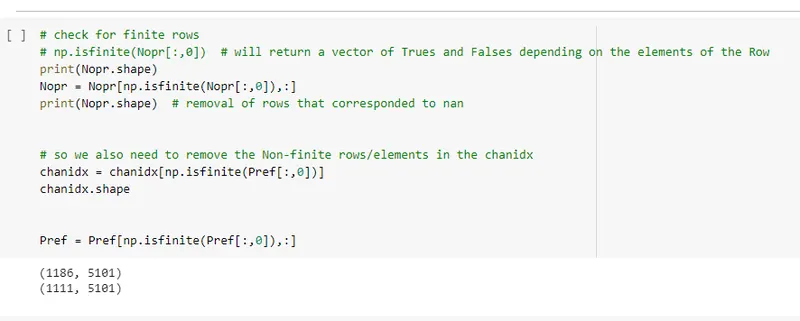
Fig: using isfinte() to keep only the rows that have the data while dropping the rest

we see that the rows are reduced from 1186 to 1111 which means only 1111 timeseries had useful information while rest were empty.

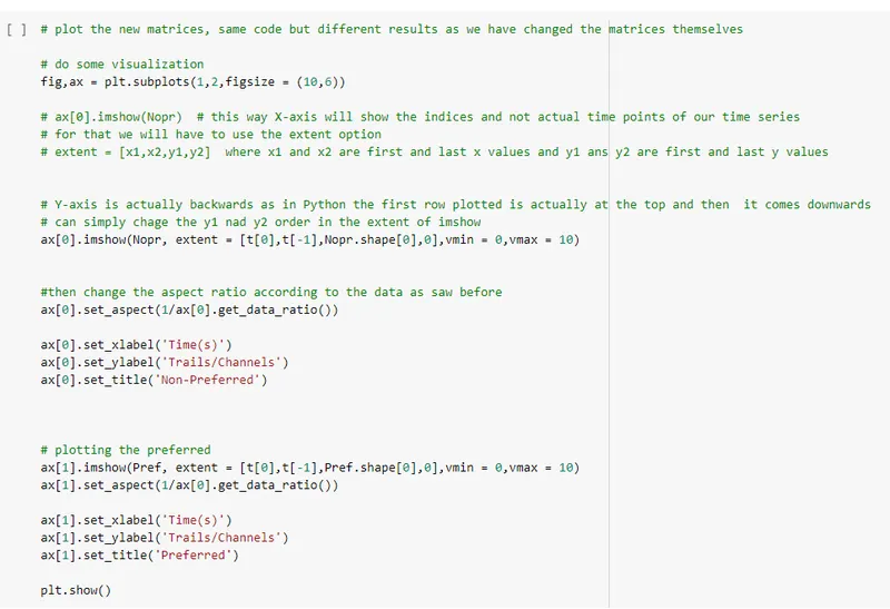
Fig: plotting the 'cleaned' data (data with no empty timeseries)

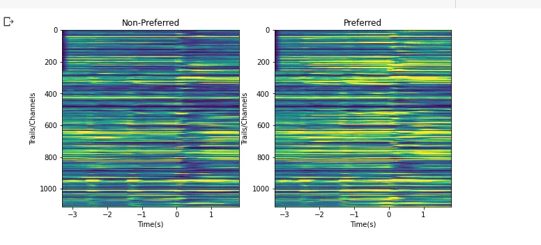
Fig: Result of the plot (with another color limit than before)

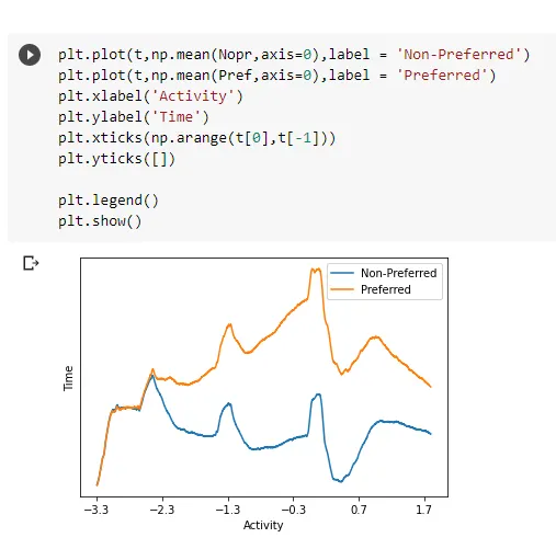
Fig: plotting the average of the time series in the rows of Preffered Data Matrix and non-Preffered Data matrix

Part II: Creating the channel by channel covariance matrix for PCA

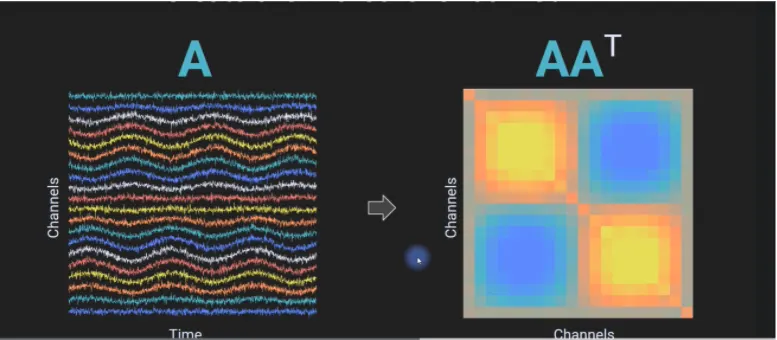
Fig: represntation of Data Matrix and covarianc ematrix

what the covariance matrix tells us?

Each element in the covariance matrix shows the correlation between the 2 channels (ith and jth channel) for the ijth element .They are very useful because they pack a lot of information into a compact form.

Approach taken:

• we have 2 data matrices
• we will compute the covariance matrix of both of them
• then take the average of the 2 covariance matrix(one from pref other non-pref)
• perfrom PCA on the new Averaged cov matrix

we will have to first create new data matrix as :

• current matrix has 1186 rows but channels are only 64
• this is because we have multiple trials of same newuron
• first we will average over the trails of each single neuron
• then we will end up with 64*5101 matrix
• from that we will create the channel covariance matrix of 64*64

so each row in the 64*5101 will represent the average response of each single neuron.

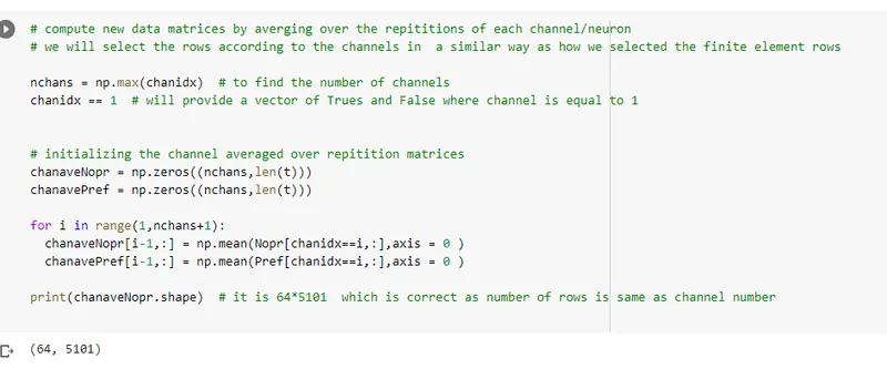
Fig: code to average over the different trails of each of the 64 neurons and then storing the mean of that in a new row

we see we avearge over the different trials and ended up with 64*5101 data matrix. Each of the 64 row is actually the avarage response of that particular newuron over the different trials it had.

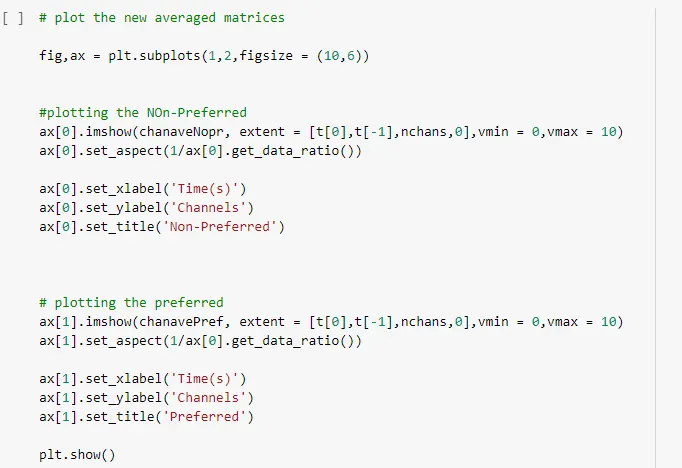
Fig: plotting the images of the new data matrices with avaeraged response of the neurons (64*5101),that is 1 row for each neuron

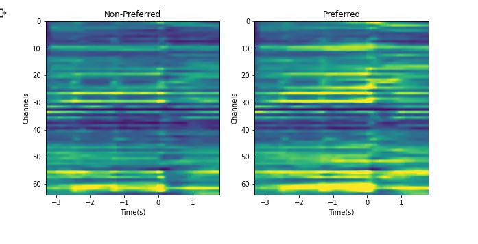
Fig: we ended up with new data matrices of 64 rows for both the Preferred and Non-Preffered Data Matrices

Part III: Computing the Channel Covariance matrices:

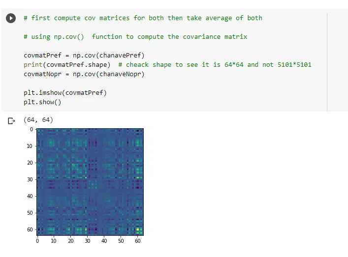
Fig : code to compute the covariance matrix of both the data matrices using np.cov(), figure shows the cov mat of Preffered data matrix

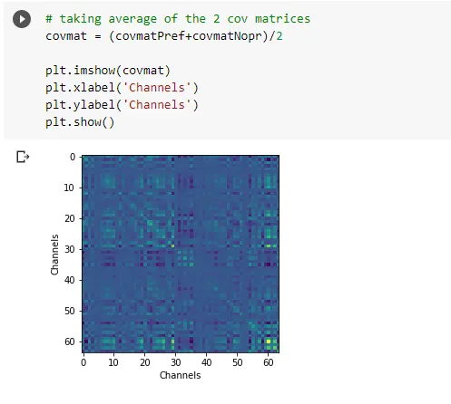
Fig: Averaging the 2 covariance matrices of Preffered and Non-Prefferes and displaying its image

Part IV : PCA on the Average channel covariance matrix:

PCA is nothing but the eigen decomposition of the Covariance matrix.

Eigen decomposition leads to breaking of the matrx into the Eigen vectors and Eigen values

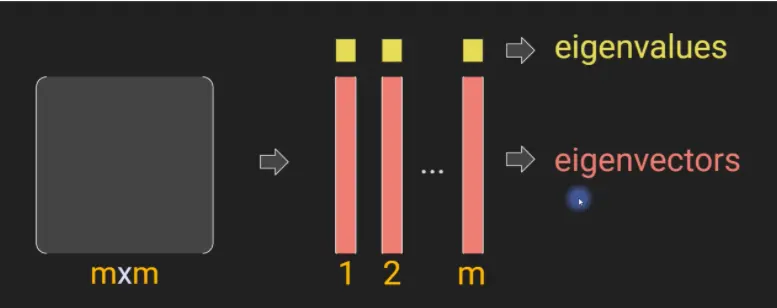
Fig: illustration of breaking a (m*m) square matrix into set of m eigen vectors and eigen values

Idea is: eigen vectors point in important directions in the space of the matrix and the eigen values tell us how important a particular direction/vector is

then we find the most important eigen vectors by plotting the eigen values.

more the magnitude of the eigen value more importtant in the corresponding eigen vector

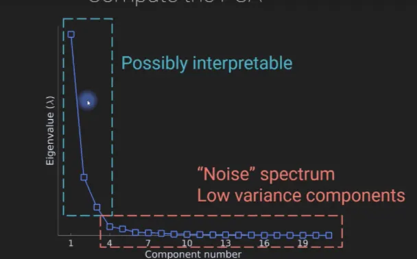
Fig: plotting the eigne values in a descending order

this is also called a Scree Plot in statistics.

Interpretation: large values eigen vealues are important and relevant to the analysis. relevant ones. While the smaller ones are not that important or relavant or maybe even noise, hence called the noise spectrum. So we eliminate the information corresponding to the eigen vectors with low eigne values and reduce the 'dimention' of the data. Also called dimention reduction.

For calculating the Principal component all we have to do is multiply the particular vector with the corresponding data matrix and then we will get the Principal component. in other words we will get the weighted sum of the rows of the data matrix where the weight are actually elements of the vector.

performing eigen decomposition using np.eigh()

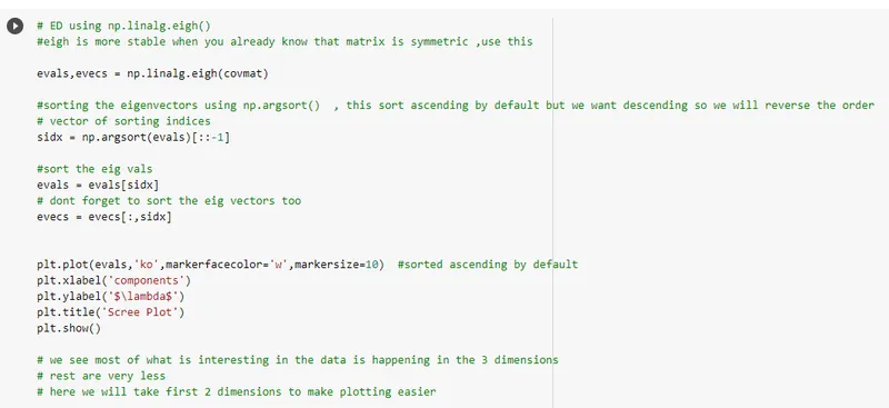
Fig: eigen decomposition of the Avergae channel covariance matrix and then arranging then eigen values and corresponding eigen vectors in descending order.

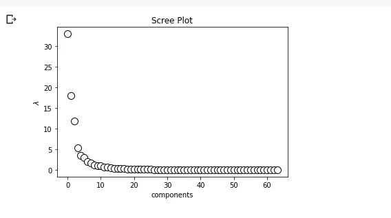
Fig: Scree plot for the eign vectors. we see 3 components are very significant than the rest 61 components

for simplicity we will only take first 2 biggest components.

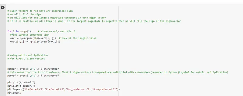
Fig: calculation of the forst 2 principal components for both the Preffered and Non_preffered Data mtrix

notice that eigen vectors by definition are negligible in length and do not have an intrinsic direction so we will have to fix the sign of the eigen vector according to the largest eigen vector

then do the vector matrix multiplication to get the Principal compents .

we take only first 2 eigen vectors for first 2 principal components

plotting the first 2 principal components of both the Data Matrices

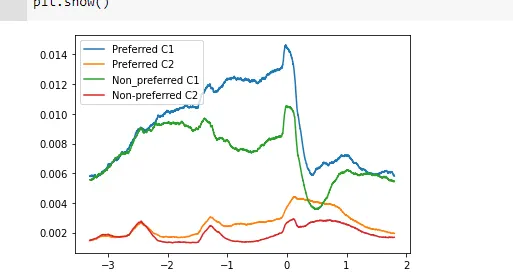
Fig: PC1 and PC2 for the Preffered and Non-Preffered Data Matrices