Solving the steady and unsteady 2D heat conduction problem
AIM
The aim of this project is to solve the 2D heat conduction equation in both steady and Transient conditions.
OBJECTIVES
To solve the 2D heat conduction equation in both steady and transient conditions.
Implement Jacobi, Gauss Sidel, Successive overrelaxation methods to solve the implicit method of the transient state analysis.
PROCEDURE
The boundary equations given for the domain are
Top Boundary = 600 K; Bottom Boundary = 900 K; Left Boundary = 400 K.
Right Boundary = 800 K.
The 2D heat conduction has 2 conditions steady and transient
We first look at the steady-state conditions.
STEADY STATE is a condition where a particular quantity does not change with time. In this case, the temperature is not dependant on time.
Let us first look at the 2D heat conduction equation.∂2T∂x2+∂2T∂y2=1α∂T∂t">
`(∂^2 T)/(∂x^2 )+(∂^2 T)/(∂y^2 )=1/α ∂T/∂t`
For steady state, the time term gets eliminated i.e., `(∂T)/(∂t)=0 ⇒ ∇⋅T = 0`
Hence, we remain with the RHS i.e.,`(∂^2 T)/(∂x^2 )+(∂^2 T)/(∂y^2 ) = 0`, This will be referred to as the space term from here on. The space term if we observe is in the elliptic form which means it would require information from all the surrounding points hence
We can rewrite the above equation as
`(T_L-2T_P+T_R)/(Δx^2 )+(T_T-2T_p+T_B)/(Δy^2 )=0`
In the above equation L refers to left and R right, P refers to the point we are calculating the temperature for, T top B bottom.
We rearrange the above equation to find out the Tp term we get
`(2T_p)/(Δx^2 )+(2T_p)/(Δy^2 )=((T_L+T_R ))/(Δx^2 )+((T_T+T_B ))/(Δy^2 )`
`T_p (2(Δx^2+Δy^2 )/(Δx⋅Δy))=(T_L+T_R)/(Δx^2 )+(T_T+T_B)/(Δy^2 )`
Let, `k=2(Δx^2+Δy^2 )/(Δx^2⋅Δy^2 )`
`T_p=1/k ((T_L+T_R)/(Δx^2 )+(T_T+T_B)/(Δy^2 ))`
Now the above equation can be solved using iterative solvers. We look at solving the above equation using Jacobi, Gauss-Sidel, SOR.
More information about the actual procedure of these methods can be found in any standard engineering mathematics textbooks and online.
Now we convert this into MATLAB/Octave program.
The code will look something like this
clear all
close all
clc

%d^2 T/ dx^2 + d^2 T/dy^2 = 0

%The above equation is still a linear PDE hence we can use either iterative or
%direct numerical methods to solve this equation.
%This equation is in the form of an elliptical PDE
%it takes data inputs from all the surrounding points

%we assume that the domain is a unit square
%L = 1
%assume some number of grid points to find out x and y using the linspace command
%Assume nx = ny
%initial conditions need to be given by the programmer
%a good initial condition will help the algorithm to complete the process faster
%since the left temperature of the temperature is given as 400k i assume the same
%the initial conditions would be T1 = 400K
%in the constructed domain the left side temp all along the y axis would be Tl = 400k
%similarly the right side nx =10 all along y would be 800k

%inputs

%Given the error should'nt be greater than
tol_given = 1e-4;

%defining grid spacing
nx = 10;
ny = 10;

%defining x and y
x = linspace(0,1,nx);

y = linspace(0,1,ny);

%defining the value of dx and dy
dx = x(2) - x(1);
dy = y(2) - y(1);

%%%%///////intial conditions///////
T = 400*ones(nx,ny);
%boundary conditions
T(:,10) = 800;
T(:,1) = 400;
T(1,:) = 600;
T(10,:) = 900;
%According the boundary condition we find out the temperature at the
%border points by finding out the mean of the temeperatures at two
%adjacent boundaries
T(1,10) = 700;
T(1,1) = 500;
T(10,1) = 650;
T(10,10) = 850;

%saving the intial  temperature in another variable just in case we
%perform any operations on the original temperature values
Told = T;
Tinitial = T;

%we reduce the complexity of the formula by predefining some terms
k = ((dx^2)*(dy^2))/(2*((dx^2)+(dy^2)));

%iterative_solver input will decide as to which method is to be used for
%calculation
iterative_solver = 3;
%defining the error term
error_term = 9e9;

%Jacobi method

if iterative_solver == 1
  jacobi_iter_num = 1;
  while error_term > tol_given
    for i =2:nx-1
      for j = 2:ny-1
        %since the boundary conditions are known the first and last terms
        %are known hence we do not calculate them here
        term1 = (Told(i-1,j)+Told(i+1,j))/(dx^2);
        term2 = (Told(i,j-1)+Told(i,j+1))/(dy^2);
        T(i,j) = k*(term1+term2);
      end
    end
    error_term = max(max(abs(Told - T)));%updating the error term
    Told = T;%updating the Told value
    jacobi_iter_num = jacobi_iter_num + 1;% counting the number of iterations required
  end
  figure(1)
  hold on
  contourf(x,y,T,'showtext','on')
  set(gca,'ydir','reverse')
  colorbar
  colormap(jet)
  grid on
  xlabel('X')
  ylabel('Y')
  title_text = sprintf('Jacobi method, iteration number is %d',jacobi_iter_num);
  title(title_text)
  pause(0.03)
end

%Guass Sidel method

if iterative_solver == 2
  GS_iter_num = 1;
  while error_term > tol_given
    for i =2:nx-1
      for j = 2:ny-1
        term1 = (T(i-1,j)+T(i+1,j))/(dx^2);
        term2 = (T(i,j-1)+T(i,j+1))/(dy^2);
        T(i,j) = k*(term1+term2);
      end
    end
    error_term = max(max(abs(Told - T)));
    Told = T;
    GS_iter_num = GS_iter_num + 1;
  end
  figure(2)
  hold on
  contourf(x,y,T,'showtext','on')
  set(gca,'ydir','reverse')
  colorbar
  colormap(jet)
  grid on
  xlabel('X')
  ylabel('Y')
  title_text = sprintf('Gauss Sidel Method, iteration number is %d',GS_iter_num);
  title(title_text)
  pause(0.03)
end

%Successice Over Relaxation method
%for the successive over relaxation method we need to define the omega
%value. Usually the values such as 1.9 or above will result in the solution
%not converging hence we use values near to 1.2
%omega
omega = 1.2;

if iterative_solver == 3
  iter_num = 1;
  while error_term > tol_given
    for i =2:nx-1
      for j = 2:ny-1
        term1 = (T(i-1,j)+T(i+1,j))/(dx^2);
        term2 = (T(i,j-1)+T(i,j+1))/(dy^2);
        %T(i,j) = ((1-omega)*Told(i,j)) + (omega*((k)*(term1+term2)));
        T(i,j) = k*(term1+term2);
      end
    end
    error_term = max(max(abs(Told - T)));
    Told = T;
    iter_num = iter_num + 1;
  end
  figure(3)
  hold on
  contourf(x,y,T,'showtext','on')
  set(gca,'ydir','reverse')
  colorbar
  colormap(jet)
  grid on
  xlabel('X')
  ylabel('Y')
  title_text = sprintf('Successive Over Relaxation Method, iteration number is %d',iter_num);
  title(title_text)
  pause(0.03)
end
Plots
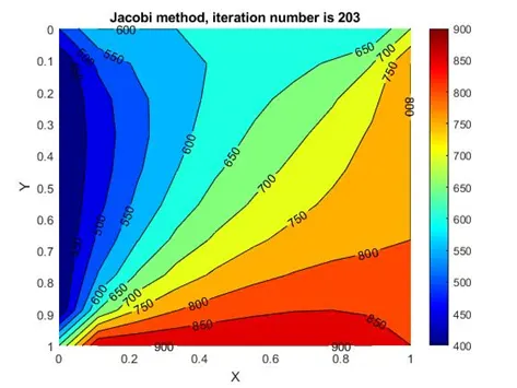
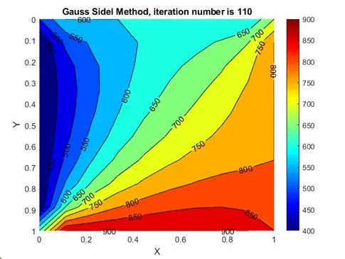
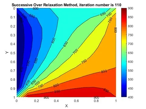
Now that we found the temperature at various nodes in a steady-state let us find out the same in a transient state.
A transient state is a condition in which Temperature changes with respect to time.
So here the time term does not vanish i.e., `(∂T)/(∂t)≠0`
So, the 2D heat conduction equation for a transient state would become
`(∂T)/(∂t)-α((∂^2 T)/(∂x^2 )+(∂^2 T)/(∂y^2 ))=0`
Since the space term is elliptic it takes input from all the adjacent points
If we apply the time marching method, then the equation would become
`(T_(i,j)^(n+1)-T_(i,j)^n)/Δt-α((∂^2 T)/(∂x^2 )+(∂^2 T)/(∂y^2 ))=0`
Now according to the time step we assume for the space term, the above equation is divided into two forms
- Explicit
- Implicit
In the explicit method, we assume time step n, this is solved in the following method
`(T_(i,j)^(n+1)-T_(i,j)^n)/(Δt)-α((T_(i+1,j)^n-2T_(i,j)^n+T_(i-1,j)^n)/(Δx^2 )+(T_(i,j+1)^n-2T_(i,j)^n+T_(i,j-1)^n)/(Δy^2 ))=0`
`T_(i,j)^(n+1)=T_(i,j)^n+αΔT((T_R^n-2T_p^n+T_L^n)/(Δx^2 )+(T_T^n-2T_p^n+T_B^n)/(Δy^2 ))=0`
Let, `CFL_x=k_1=α (Δt)/(Δx^2 )` and `CFL_y=k_2=α(Δt)/(Δy^2 )`
Where CFL is called the courant number which is just a dimensionless number that specifies how much fluid has passed in a particular cell, this matters a lot in explicit methods for care should be taken while taking inputs such that the courant number lies below 0.5. If the courant number is above 0.5 then the solution would be unstable. The equation becomes
`T_(i,j)^(n+1)=T_(i,j)^n+K_1 (T_R^n-2T_p^n+T_L^n )+k_2 (T_T^n-2T_p^n+T_B^n )`
In the implicit methods, we consider (n+1)th time step for the space term and can be solved using the iterative solvers. Before using the iterative solvers let us first simplify the equation
`T_(i,j)^(n+1)=T_P^(n+1)=T_P^n+αΔt((T_R^(n+1)-2T_P^(n+1)+T_L^(n+1))/(Δx^2 )+(T_T^(n+1)-2T_P^(n+1)+T_B^(n+1))/(Δy^2 ))`
Let`k_1=α(Δt)/(Δx^2 )` and`k_2=α(Δt)/(Δy^2 )`
`T_p^(n+1)=T_P^n+K_1 (T_L^(n+1)-2T_P^(n+1)+T_R^(n+1) )+K_2 (T_T^(n+1)-2T_p^(n+1)+T_B^(n+1) )`
`T_p^(n+1)-k_1 T_L^(n+1)+2k_1 T_p^(n+1)-k_1 T_R^(n+1)-K_2 T_T^(n+1)+2k_2 T_P^(n+1)-k_2 T_B^(n+1)=T_p^n`
`T_p^(n+1) (1+2k_1+2k_2 )-k_1 T_L^(n+1)-k_1 T_R^(n+1)-k_2 T_T^(n+1)-k_2 T_B^(n+1)=T_p^n`
`T_p^(n+1)=(T_p^n+K_1 T_L^(n+1)+k_1 T_R^(n+1)+k_2 T_T^(n+1)+k_2 T_B^(n+1))/((1+2k_1+2k_2 ) )`
`T_p^(n+1)=(T_p^n+k_1 (T_L^(n+1)+T_R^(n+1) )+k_2 (T_T^(n+1)+T_B^(n+1) ))/((1+2k_1+2k_2 ) )`
The term `T_p^n` stays constant with each iteration, it will change only when there is a change in time step.
Now that we have derived the necessary equations let us convert the above into a MATLAB/Octave program.
The code would look something like this
clear all
close all
clc

%defining grid spacing
nx = 10;
ny = 10;

%Given the error shouldn't be greater than
tol_given = 1e-4;

%defining x and y
x = linspace(0,1,nx);
y = linspace(0,1,ny);

%defining the value of dx and dy
dx = x(2) - x(1);
dy = y(2) - y(1);

%%%%///////intial conditions///////
T = 400*ones(nx,ny);
%boundary conditions
T(:,ny) = 800;
T(:,1) = 400;
T(1,:) = 600;
T(nx,:) = 900;
%defining temperature at corner points
T(1,ny) = 700;
T(1,1) = 500;
T(nx,1) = 650;
T(nx,ny) = 850;

%saving the initial values using another variable
Told = T;
%defining the T at previous time step
T_prev_dt = Told;

%this part defines what solver to be used
sssE = 0;
iter_sol_num = 3 ;

%Now that we finished the steady-state analysis
%we move on to transient analysis
%This can be solved using two methods
%explicit and implicit methods

%Solving using the explicit method
%here we have to observe the courant number
%CFLx K1 = alpha(dt/dx^2) ; CFLy K2 = alpha(dt/dy^2)
%for explicit methods CFL <= 0.5
%{CFLx + CFLy <= 0.5}
%if the courant number value is greater than specified the solution never converge.
%so we give time inputs such that the courant number value is maintained.
%since time is introduced we introduce the time frame term
%the total number of timesteps
nt = 1400;
%difference between timesteps
dt = 0.0025;

%introducing the alpha term
alpha = 1.4;

%from alpha, dt, dx, dy we calculate the courant numbers
k1 = alpha*dt/(dx^2);
k2 = alpha*dt/(dy^2);

if sssE == 1
  for nt = 1:1400%for all timesteps
    for i = 2:nx-1%for all the nodes except the starting and the ending nodes
      for j = 2:ny-1
        T(i,j)=T(i,j) + k1*(T(i-1,j)-(2*T(i,j))+T(i+1,j)) + k2*(T(i,j+1)-(2*T(i,j))+T(i,j-1));
      end
    end
  end
  figure(3)
  hold on
  contourf(x,y,T,'showtext','on')
  set(gca,'ydir','reverse')
  colorbar
  colormap(jet)
  grid on
  xlabel('X')
  ylabel('Y')
  title_text = sprintf('Transient state explicit method');
  title(title_text)
end

%Now we got the solution using the explicit method, let's try obtaining the solution
%to the same using the implicit method
%in the implicit method the courant number won't affect much, we can leave the time inputs unchanged
% but since the system of equations grows complex we use the iterative solvers to
%solve the system of equations
%we will use the simplified equation in the program

%Jacobi method
if iter_sol_num == 1
  jacimplnum = 1;
  for nt = 1:1400
      error_term = 100;%The error term is defined at this point if it is not defined here****
    while error_term > tol_given
      for i = 2:(nx-1)
        for j = 2:(ny-1)
          term1 = 1/(1+(2*k1)+(2*k2));%for simplification of equation we predefine some terms
          term2 = k1*term1;
          term3 = k2*term1;
          H = (Told(i-1,j)+Told(i+1,j));
          V = (Told(i,j-1)+Told(i,j+1));
          T(i,j) = (T_prev_dt(i,j)*term1)+(H*term2)+(V*term3);
        end
      end
      error_term = max(max(abs(Told-T)));%updating the error term two max are used so as to obtain a single value
      Told = T;%updating Told
      jacimplnum = jacimplnum + 1;  %counting the number of iterations
    end
    T_prev_dt = T;  %the tprev will be constant through out the while loop it gets updated at the end of time loop
  end
  figure(1)%plotting the t values if the plot is made in the time loop it would take a while
  contourf(x,y,T,'showtext','on')
  set(gca,'ydir','reverse')%this will reverse the
  colorbar
  colormap(jet)
  grid on
  xlabel('X')
  ylabel('Y')
  title_text = sprintf('Jacobi method, iteration number is %d',jacimplnum);
  title(title_text)
end

%******Then the error term gets updated after each time step and a valid
%solution won't arrive but the process will be completed in less number of
%iterations

%GAUSS SIDEL METHOD
if iter_sol_num == 2
  GSnum = 1;
  for nt = 1:1400
      error_term = 100;
    while error_term > tol_given
      for i =2:(nx-1)
        for j = 2:(ny-1)
          term1 = (1+(2*k1)+(2*k2))^-1;
          term2 = k1*term1;
          term3 = k2*term1;
          H = (T(i-1,j) + Told(i+1,j));
          V = (T(i,j-1) + Told(i,j+1));
          T(i,j) = ((T_prev_dt(i,j))*term1)+(H*term2)+(V*term3);
        end
      end
      error_term = max(max(abs(Told - T)));
      Told = T;
      GSnum = GSnum + 1;
    end
    T_prev_dt = T;
  end
  figure(1)
  contourf(x,y,T,'showtext','on')
  set(gca,'ydir','reverse')
  colorbar
  colormap(jet)
  grid on
  xlabel('X')
  ylabel('Y')
  title_text = sprintf('Gauss Sidel method, iteration number is %d',GSnum);
  title(title_text)
end

if iter_sol_num == 3
  SORnum = 1;
  omega = 1.2;
  for nt = 1:1400
      error_term = 100;
    while error_term > tol_given
      for i = 2:(nx-1)
        for j = 2:(ny-1)
          term1 = (1+(2*k1)+(2*k2))^-1;
          term2 = k1*term1;
          term3 = k2*term1;
          H = (T(i-1,j) + Told(i+1,j));
          V = (T(i,j-1) + Told(i,j+1));%note that if we used the Gauss sidel temperature here
          T_GS(i,j) = ((T_prev_dt(i,j))*term1) + (H*term2) + (V*term3);
          T(i,j)=((Told(i,j))*(1-omega))+(omega*(T_GS(i,j))); %SOR temperature
        end
      end
      error_term = max(max(abs(Told - T)));
      Told = T;
      SORnum = SORnum + 1;
    end
    T_prev_dt = T;
  end
  figure(3)
  contourf(x,y,T,'showtext','on')
  set(gca,'ydir','reverse')
  colorbar
  colormap(jet)
  grid on
  xlabel('X')
  ylabel('Y')
  title_text = sprintf('Succesive over relaxation method, iteration number is %d',SORnum);
  title(title_text)
end
Plots obtained
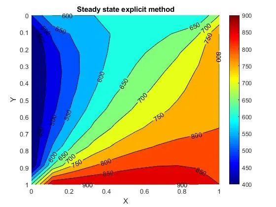
(The above picture has been wrongly titled. It is the plot of transient state explicit method)
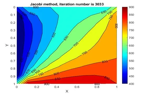
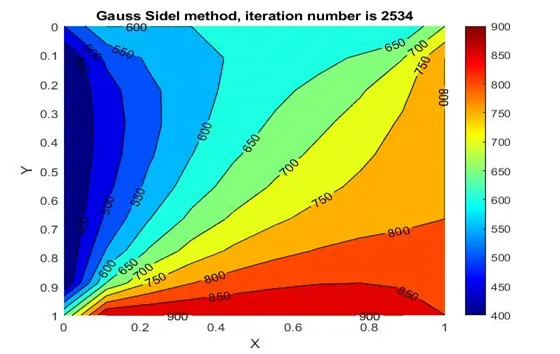
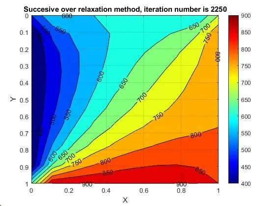
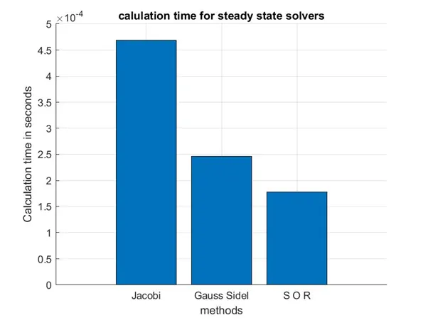
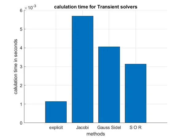
For the steady-state analysis, the tic and toc commands were placed before and after the convergence loop. And the time taken for different iterative solvers are as follows
|
Steady State |
|
|
S O R |
0.0018 |
|
G S |
0.0021 |
|
Jacobi |
0.0044 |
|
Unsteady State |
|
|
explicit |
0.0045 |
|
Jacobi |
0.0114 |
|
G S |
0.0092 |
|
S O R |
0.0076 |
For transient state, we placed the tic and toc commands in before and after the time loop and the time taken for different iterative solvers are as shown above
The below plots show the calculation time required for each method in both steady and transient methods.
CONCLUSION
- From the above graphs, we can see that for the same temperature profile the number of iterations required differs for different iterative methods
- The number of iterations required for Jacobi > Gauss-Sidel > SOR. This implies because the solution converges early in the SOR method compared to the other two methods.
- In the Steady-state the SOR method converges much early compared to the other two methods. While in the transient state the explicit method converges much faster than the implicit methods. In the implicit methods, the SOR method converges at an early rate compared to Jacobi and Gauss Sidel methods.
- The accuracy of the solution doesn't seem to differ with the method used but the time required to attain that accuracy changes.
- For this project, the time varies within milliseconds but for huge problems, the time may vary in minutes or even hours.
- In a steady-state condition should we require less calculation time with more accuracy we can go for the SOR method.
- In a transient state if we require less calculation time with good accuracy we can go for the explicit method or SOR in implicit methods.
- Also, on experimentation with the dt it is observed that as we reduce the dt the number of iteration required increases.