Project

Solving second order ODE's : Simple Pendulum

AAnup Deshmukh16 May 2020

Solving Second Order ODE's in MATLAB : Simple Pendulum

1. AIM:

To solve a second order ordinary differential equation in matlab.

2. GOVERNING EQUATIONS:

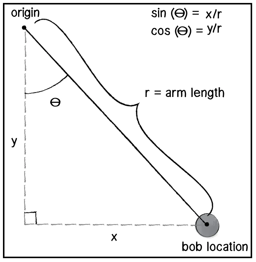
Fig 1: Trigonometry relations for a simple pendulum

Variables:

- $\theta$ θ is the angle made by rod with vertical

- B is damping coefficient

- m and L are mass of the bob and length of the rod / string

1. $\frac{d^{2} θ}{d t^{2}} + \frac{b}{m} \frac{d θ}{d t} + \frac{g}{L} s i n θ = 0$ \dfrac {d^2\theta} {dt^2} + \dfrac b m \dfrac {d\theta}{dt} + \dfrac g L sin\theta = 0dt2d2θ+mbdtdθ+Lgsinθ=0 Second order ODE. -------(1)

To solve this, we need to reduce it into lower order ODE by substitution. thus,

let $θ = θ_{1}$ \theta = \theta_1θ=θ1

So, we can say that $\frac{d θ}{d t} = \frac{d θ_{1}}{d t} = θ_{2} (s a y)$ \dfrac {d\theta}{dt} = \dfrac{d\theta_1}{dt} = \theta_2 (say)dtdθ=dtdθ1=θ2(say) ------(2)

Therefore, $\frac{d^{2} θ}{d t^{2}} = \frac{d^{2} θ_{1}}{d t^{2}} = \frac{d}{d t} (\frac{d θ_{1}}{d t}) = \frac{d}{d t} (θ_{2})$ \dfrac {d^2\theta}{dt^2} = \dfrac{d^2\theta_1}{dt^2} = \dfrac{d}{dt}(\dfrac{d\theta_1}{dt}) = \dfrac{d}{dt}(\theta_2)dt2d2θ=dt2d2θ1=dtd(dtdθ1)=dtd(θ2) ------(3)

Putting (2) and (3) in (1), we get :

$\frac{d^{2} θ_{1}}{d t^{2}} + \frac{b}{m} \frac{d θ_{1}}{d t} + \frac{g}{L} s i n (θ_{1}) = 0$ \dfrac{d^2\theta_1}{dt^2} + \dfrac{b}{m}\dfrac{d\theta_1}{dt} + \dfrac{g}{L}sin(\theta_1) = 0dt2d2θ1+mbdtdθ1+Lgsin(θ1)=0 that is

$\frac{d θ_{2}}{d t} + \frac{b}{m} θ_{2} + \frac{g}{L} s i n θ_{1} = 0$ \dfrac{d\theta_2}{dt} + \dfrac{b}{m}\theta_2 + \dfrac{g}{L}sin\theta_1 =0dtdθ2+mbθ2+Lgsinθ1=0

Since it is reduced to lower order, by rearranging terms, we can say that, $\frac{d θ_{2}}{d t} = - \frac{b}{m} θ_{2} - \frac{g}{L} s i n θ_{1}$ \dfrac{d\theta_2}{dt} =- \dfrac{b}{m}\theta_2 - \dfrac{g}{L}sin\theta_1dtdθ2=−mbθ2−Lgsinθ1

3. OBJECTIVES OF THE PROJECT:

- To solve the second order ODE in MATLAB with graphs for velocity and displacement.

- To simulate the motion of simple pendulum in MATLAB.

4. FLOW OF THE PROJECT:

- Lower the order of the ODE using substitution method. Prepare a function for the same for code neatness purpose.
- Set the geometrical and physics parameters of the pendulum like length, mass, damping coefficient as well as gravity.
- Set the initial conditions and timespan for which you want to run the simulation.
- Use the inbuilt ODE solver named ODE45 to solve the ODE which is reduced by calling our function that is made in step 1 and obtain values of displacement and velocity and store it in an array.
- Plot the graph of displacement v/s time and velocity v/s time.
- Create simulation of the positions of the pendulum bob and arm using movie function.
5. MATLAB CODE:
Code for the function of ode reduction

function [dtheta_dt] = ode_func(t,theta,b,g,l,m)

theta1 = theta(1);
theta2 = theta(2);
dtheta1_dt = theta2;
dtheta2_dt = -(b/m)*theta2 - (g/l)*sin(theta1);
dtheta_dt = [dtheta1_dt; dtheta2_dt]

end

Code explaination:
- Refer the section 2 of the report named GOVERNING EQUATIONS. The steps followed in the section 2 have been converted into matlab code likewise.
- The only addition is that the final derivation of theta1 and theta2 is stored in an array because of presence of multiple values.
Code for the main program

clear all
close all
clc

%given conditions of length, damping coeff, mass and gravity accleration
b=0.05;
g=9.81;
l=1;
m=1;

%initial conditions
theta_0 = [0,3];   %[angle displacement,velocity]

%time spans
t_span=linspace(0,20,1000);

%ode solver
[t,results] = ode45(@(t,theta) ode_func(t,theta,b,g,l,m),t_span,theta_0);

figure(1)
plot(t,results(:,1))       %plot all rows from first column
hold on                    %retain all the data from first plot
grid on
plot(t,results(:,2))       %plot all rows from second column
axis([0 20 -3 3])          %resize the graph to show X and Y axis from/to X,X(0,20) and Y,Y(-3,3)
ylabel('Plot')
xlabel('Time')


x0=1;                      %to set a hinge point
y0=1;
ct=1;
coord = results(:,1);      %all rows from first column which are angle values

for i=1:length(coord)  
figure(2)                 %open in new window, new figure
x1 = 1-l*sin(coord(i));    %x coordinate from trigonometry
y1 = 1-l*cos(coord(i));    %y coordinate from trigonometry
plot([0,2],[1,1],'linewidth',5)          %a support line for hinge (not necessary)
hold on
plot([1,x1],[1,y1],[x1,x1],[y1,y1],'o','MarkerFaceColor','r','linewidth',2)      %plotting lines from hinge to the end with a ball marker at the end
hold off
axis([0 2 -0.5 1.5])
grid on
pause(0.01)

M(ct) = getframe(gcf);
ct = ct+1;

end

movie(M)                        %starting to create a video file
videofile = VideoWriter('pendulum.avi','uncompressed AVI');      %creating a video file named pendulum with avi extension
open(videofile)                 %open the video file
writeVideo(videofile,M)         %write the plot images to the fideo file
close(videofile)                %close the video file.

Code explaination:
1. Set physics parameters of the pendulum like mass, length, gravity and damping coefficient.
2. Set the initial conditions and timespan for which you want to run the simulation.
3. To use the ode solver, use ode45 function with main inputs as (t and theta) while you use ode_func (the one we created earlier) with inputs as (t,theta,l,b,g,m) and t_span and theta_o as the initial conditions.
4. These results are stored in an array of [t,results]
5. Since results contain 2 components, angle displacement and velocity, to plot both the graphs, use the (:,1) and (:,2) property of MATLAB and plot those graphs.
6. To create animation, Use a for loop so that we can get X and Y co-ordinates using trigonometry, Here, x0 and y0 are the hinge points. Since they are (1,1) we have subtracted the co-ordinates of the bob from them so that proper rod of the pendulum can be seen.
7. Use the pause () function to give a pause for every looping of values.
8. Use movie making commands as per code to create a animation video.
6. ERRORS FACED:
Error #1
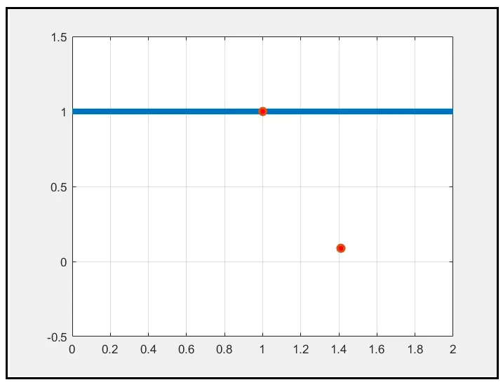
The string or the rod of the pendulum was not visible. Fixed it by putting the marker dot in the initial plot itself, and not in another
.Error #2
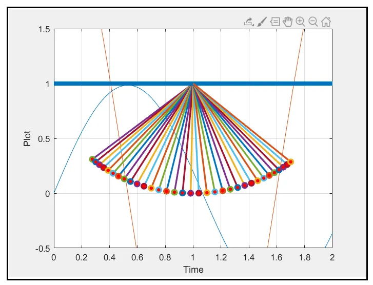
Here, the problem was when we switched the tab from second plot(animation) to the first plot (displacement,velocity), the animation was overlapping.
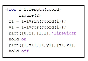
Fixed it by putting the figure(2) inside the for loop (previously it was outside the for loop) and fixed the multiple lines issue by using hold off command.
7. OBSERVATIONS: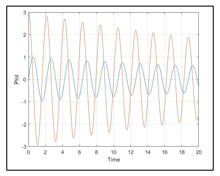
We can see that the plot of Displacement(blue color) and Velocity(red) is plotted against time. We can see the reduction of velocity and angle displacement as time increases.
8. CONCLUSION:
- The reduction in velocity and Angle displacement is due to damping coefficient introduced in the Second order ODE of a simple pendulum.
- We have successfully solved the second order ODE.
- The animation of the pendulum is here https://youtu.be/OIw_YrWja1E