Plotting Air Standard Cycle (Otto Cycle) in MATLAB

Air Standard Cycle (Otto Cycle)

1.AIM:

· To plot the Air standard cycle (Otto cycle) for Pressure v/s Volume using MATLAB.

2.GOVERNING EQUATIONS IF ANY:

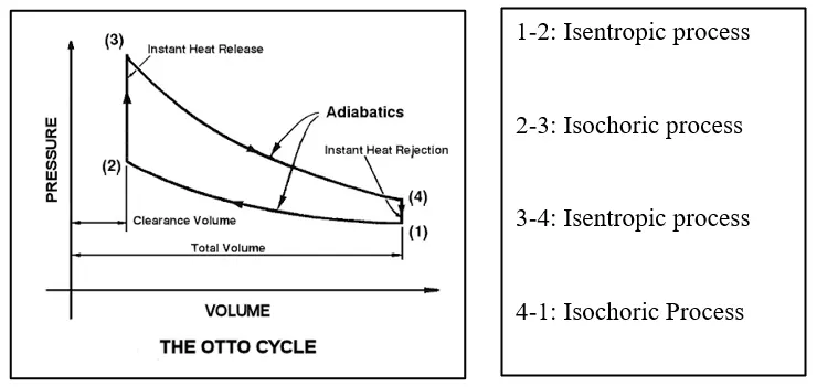
· For Isentropic process 1-2 and 3-4:

$P_1 V_1^γ=P_2 V_2^γ$P1​V1γ​=P2​V2γ​ and $(P_1V_1)/T_1 = (P_2V_2)/T_2$(P1​V1​)/T1​=(P2​V2​)/T2​

where numbers indicate the process state.

· Assumptions: 1. Sp. Heat Ratio (γ) = 1.4

2. Temp. after compression ($T_3$T3​) = 2500K

3. $P_1$P1​ = 101325 Pa

4. $T_1$T1​ = 400K

· Geometric assumptions: 1. Bore Diameter = 0.2m

2. Stroke = 0.2m

3. Compression Ratio (CR) = 12

4. Connecting rod length = 0.23m

5. $R+1-cos(θ)-(R^2-sin^2(θ))^{1/2}$V/Vc​=1+1/2(CR−1) [R+1−cos(θ)−(R2−sin2(θ))1/2]

· Where θ is the crank angle

6. Thermal efficiency = $η_{th}=1-1/CR^{γ-1}$ηth​=1−1/CRγ−1

3.OBJECTIVES OF THE PROJECT:

· To plot the air standard (Otto) cycle for Pressure v/s Volume in MATLAB.

· To find the thermal efficiency of the engine.

4.FLOW OF THE PROJECT:

i. Assume critical geometric components and initial values of pressure and temperature.

ii. Calculate values of pressure and temperature at different stages of the cycle i.e. 1 to 4 using governing equations of different types of processes being used.

iii. Plot the graphs mentioned in the objectives.

iv. Find the thermal efficiency.

5.MATLAB CODE:

Code for the function used:

%Creating a function named otto_2_piston whose output is v and input
%parameters are bore diameter, stroke length, length of connecting rod,
%compression ratio, staarting and ending crank angle.
function [v] = otto_2_piston(bore,stroke,con_rod,cr,start_crank,end_crank)
 
%geometric dimensioning
a = stroke/2;
R = con_rod/a;
 
%Swept and clearance volume 
v_s = (pi/4)*bore^2*stroke;
v_c = v_s/(cr-1);
 
%specifying an array of angles for crank angle theta
theta = linspace(start_crank,end_crank,100);
 
%for finding the volume in terms of clearance volume, compression ratio and
%geometric dimensions
term1 = 0.5*(cr-1);
term2 = R+1-cosd(theta);
term3 = (R^2-sind(theta).^2).^0.5;
v = (1+term1*(term2-term3)).*v_c;
end

· Code explanation:

1. To simplify the usage of various formulas repeatedly in the main program, we have made a small function named “otto_2_piston” so that we can recall it in the main function any number of times we want. It results in clean and neat code.

Code for the main (function utilizing) program:

clear all
close all
clc
 
%Assumptions as inputs
gamma = 1.4;
t3 = 2500;
 
%state variables at 1
p1 = 101325;
t1 = 400;
 
%engine geometric parameters 
bore = 0.2;
stroke = 0.2;
con_rod = 0.23;
cr = 12;
 
%Calculation of swept and clearance volune
v_swept = (pi/4)*bore^2*stroke;
v_clearance = v_swept/(cr-1);
v1 = v_swept + v_clearance;
v2 = v_clearance;
 
%state variables at pt 2
%p2v2^gamma = p1v1^gamma
p2=p1*cr^gamma;
 
%p1v1/t1 = p2v2/t2
t2 = p2*v2*t1/(p1*v1);
 
constant_c = p1*v1^gamma;
v_comp = otto_2_piston(bore,stroke,con_rod,cr,180,0);
p_comp = constant_c./(v_comp.^gamma);
 
%state point 3
v3 = v2;
 
%p3v3/t3 = p2v2/t2
p3 = p2*t3/t2;
 
constant_c = p3*v3^gamma;
v_exp = otto_2_piston(bore,stroke,con_rod,cr,0,180);
p_exp = constant_c./(v_exp.^gamma);
 
%state point 4
v4=v1;
%p3v3^gamma = p4v4^gamma
p4 = p3*(v3/v4)^gamma;
 
%thermal efficiency
ther_eff = 1-(1/(cr^(gamma-1)));
finaleff = ther_eff*100+"%"
 
figure(1)
hold on
grid on
plot(v1,p1,'*','color','r')
plot(v_comp,p_comp)
plot(v2,p2,'*','color','r')
plot(v3,p3,'*','color','r')
plot(v_exp,p_exp)
plot(v4,p4,'*','color','r')
plot([v2,v3],[p2,p3],'color','b')
plot([v4,v1],[p4,p1],'color','b')
 
%figure(2)
%plot([v1 v2 v3 v4],[p1 p2 p3 p4],'color','b');

· Code explanation:

1. We first assume some important parameters such as sp. Heat ratio (gamma) and Temperature at state 3 i.e. after heat addition.

2. We also assume initial pressure, temperature, and geometrical parameters.

3. Using the formula of volume of cylinder and clearance volume, we find out the swept and clearance volume.

4. Using governing equation of isentropic process, we thus find out pressure and temperature at state point 2.

5. After this, we call our function to help us to find the compression volume and pressure.

6. Similar thing is done in the case of state 3-4.

7. Thermal efficiency is found out and graph is plotted between pressure and volume.

6.OBSERVATION:

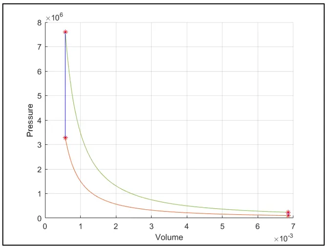
Observed the plot of each of the processes i.e isentropic, isochoric happening in the cycle between different state points

7. ERRORS FACED:

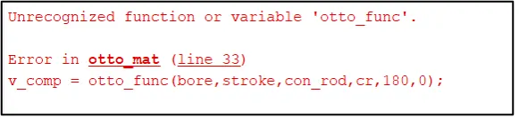
· · Did not give the name of the file same as that of the function. Fixed by renaming the file name as per the function name.

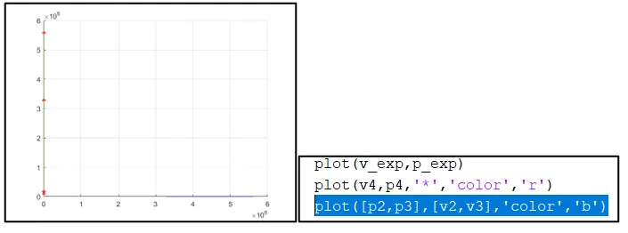
· Plotted a wrong plot where pressure was in x-axis and volume was at y-axis. So, something wrong was being plotted. Fixed by assigning proper x and y values in the plot function parameters.

8.CONCLUSION:

· Correct P-V chart of Otto cycle was plotted in MATLAB.

· Obtained thermal efficiency is 62.98%

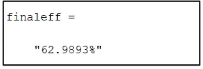
$V/V_c =1+ 1/2(CR-1$Thermal efficiency =

·