Performing Curve Fitting using MATLAB

Performing Curve Fitting using MATLAB

1. AIM:

To perform a curve fitting on a given data set using MATLAB software.

- For quadratic equations, $C_p = aT^2 + bT + c$Cp​=aT2+bT+c  and so on for other degrees of equations.

- For $R^2$R2 method,$R^2 = \dfrac{SSR}{SST}\space where \space \sum(f(x(i))-mean)^2 and\space SST = SSR + \sum(Y(i) - f(x(i)))^2$R2=SSTSSR​ where ∑(f(x(i))−mean)2and SST=SSR+∑(Y(i)−f(x(i)))2 

- For RMSE method, $RMSE = \sqrt{\dfrac{SSE}{n}}$RMSE=nSSE​​

where $a, b, c$a,b,c are coefficients of some degree of $T$T

$f(x(i))$f(x(i)) is the y coordinate of the fitted curve having equation y = f(x)

Y(i) is the y coordinate of the data set ( Cp ) here in this case.

- Read more about these formulas here.

3. OBJECTIVES OF THE PROJECT:

- Write MATLAB code to fit a linear and cubic polynomial for the Cp data

- Plotting the data and checking error using different methods

4. FLOW OF THE PROJECT:

- Collect sample data of which you want to get a curve.

- Differentiate the data and assign some variables.

- Use MATLAB to fit a polynomial degree curve through those variables and thus obtain coefficients of the variable T.

- Plot the original dataset as well as curve that is being fitted through those datasets.

- Find error so as to get an approximation of how good your curve fits the data sets.

5. MATLAB CODE:

clear all
close all
clc

%preparing the data by loading it
cp_data = load('data');
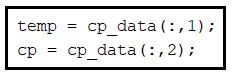
temp = cp_data(:,1);     %assigning all rows of first column as temperatures
cp = cp_data(:,2);       %assigning all rows of second column as Cp values
cftool                   %open curve fitting tool for cross checking our code

%Curve fitting

%cp = a*T^2 + b*T + c                        %quadratic equation as example
coeff = polyfit(temp,cp,2);                  %obtaining values of coefficients of the equation of some degree
predicted_cp = polyval(coeff,temp);          %putting coefficients in the original equation to get L.H.S

%compare my curve fit with original data
plot(temp,cp,'linewidth',3)                        %plotting original dataset
hold on
grid on
plot(temp,predicted_cp,'linewidth',3,'color','r')  %plotting my graph with cp which is outcome of curve fitting
xlabel('Temperature (K)')
ylabel('Specific Heat (KJ/Kmol-K)')
legend('Original dataset','My curve fit')


%checking error by R-square method
%finding the SSR
ssr=0;
sse=0;
meancp = mean(cp);                  %calculating mean of cp dataset using mean function
for i=1:length(cp)
b = (predicted_cp(i)-meancp)^2;     %looping so as to generate values of b for every value of predicted cp in dataset
ssr=ssr+b;                          %adding all the values of b
end
for j=1:length(cp)
c = (cp(j)-predicted_cp(j))^2;      %looping so as to generate value of c for every value of cp and predicted cp
sse = sse+c;                        %adding all values of c
end
sst = ssr+sse;
R = ssr/sst                         %final value of R-square

%finding RMSE
rmse = (sse/length(cp))^0.5         %final value of RMSE

Code explaination:

- First we have loaded the data given in the challenge itlself, by using load() function.

- Then we have assigned the Cp and temperature values to variables using (:,n) function because the data set is a CSV i.e Comma Seperated Values file having 2 columns, i.e. seperated by a comma.

- Then use polyfit function whose inputs will be temperature and CP and also specify what degree polynomial you will be using. here I have used 2 as the degree.

- Then using polyval function, obtain the coefficients a, b and c.

- Using plot function, plot the graph of Cp of original dataset and Predicted Cp got from puting the values obtained from the polyval into the polynomial. Compare the fit of the curve visually.

- The later part of the code is used for checking the maximum error of the fitting of the curve. 2 methods are used here, namely 1. R-square method and 2. Root mean square method.

- The value of R in R-square method should lie between 0 and 1 where 0 means poor fit and 1 means . Typically a value greater than 0.95 means a good fit.

- The RMSE value in the next method should be as less as possible to be called as a good fit.

6. ERRORS FACED:

Fixed by putting a colon (:) instead of semi-colon (;) in the (:,n) function.

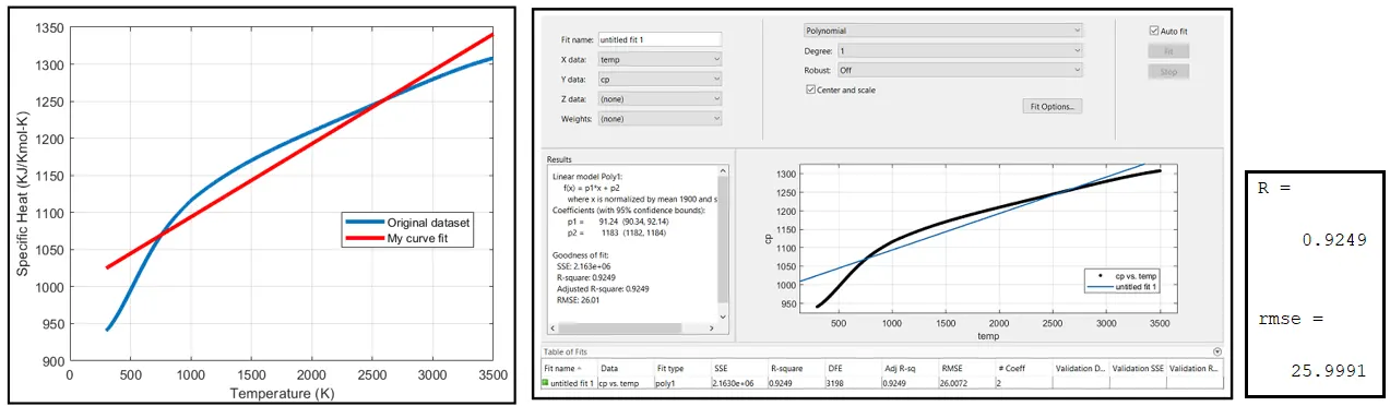
7. OBSERVATIONS:

For Linear Polynomial - Curve isn't a good fit because of high error (high value of R and rmse)

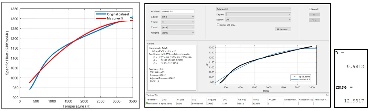
For Quadratic Polynomial - The curve is a good fit because of low value of R, 0.95<0.9812

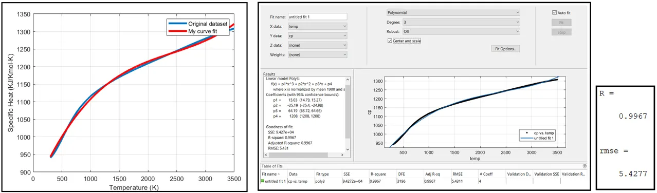
For Cubic Polynomial - The curve is better fit than quadratic polynomial because of lower R and rmse values.

For 8th order Polynomial - Perfect fit because R=1. Although rmse is 0.51, it can be lowered if we go

to 9 or more order polynomials.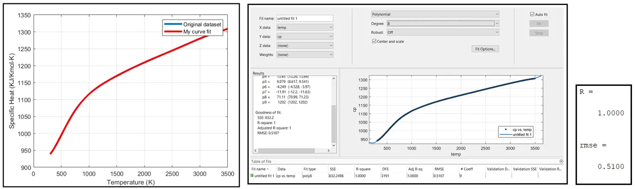

8. CONCLUSION:

- A best fit is a fit without taking errors into consideration.

- Perfect fit is the one where errors are also taken into account.

- How to improve the cubic fit?

To improve any process, reducing the size or in a simpler language, reducing the extent is must.

So to improve cubic fit, we can reduce the temperature range and make smaller segments so that it will be easy to fit the curve into smaller segments.

9. REFERENCES:

1. https://skill-lync.com/projects/Curve-Fitting-and-criterion-to-choose-best-fit-41860