Solving Second Order ODE
Objective:-
We are provided with a situation in which the coefficient of a second order ode is given. The equation provided is basically the equation of motion of a pendulum. Here damping is also considered.
Our goal is to find the position and velocity of bob of pendulum at different time in the given time span by solving the given second order ODE. Not only finding the values, we have to also plot the graphs of position and velocity versus time.
After this by using the computed data we will be creating a continuous loop describing the motion of pendulum following an animation.
Our whole process is going to be done on matlab which includes making programmes, function and make them to give required and accurate outputs.
Theory:-
Solving Second Order ODE in Damping
We are going to start our discussion on the motion of a simple pendulum going under damped oscillations. The motion will be an oscillatory and periodic motion. The equation of motion will be second order differential equation.
General equation of a second order ordinary differential equation for conditions of simple pendulum going under damped oscillations is written as:-
`d^2/dt (θ)+(b/m)*((d/dt)*θ)+(g/l)*sinθ=0`
Here,
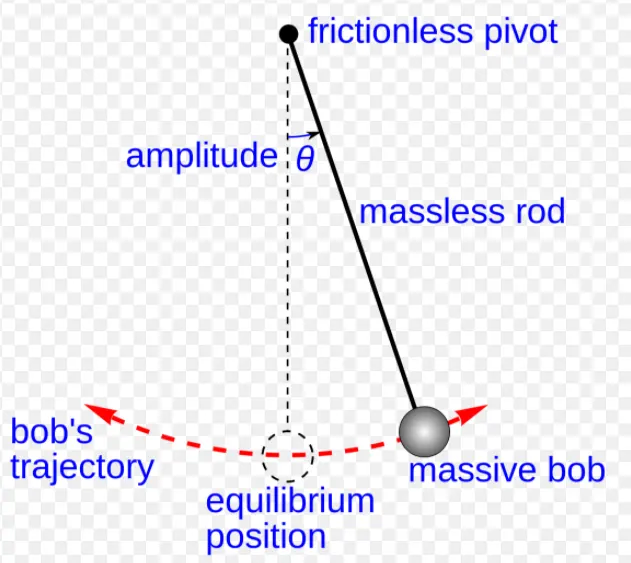
b= damping coefficient
m= mass of the bob of simple pendulum
g= gravity (9.8 m/s^2)
l= Length of string of simple pendulum
θ is the displacement of the bob from the vertical.
Now, we move on solving the equation.
Let θ=θ1 -----equation 1
Also,
`(d/dt)*θ=(d/dt)*θ1=θ2`
--------------equation 2
Therefore, the general equation can be written in terms of θ1 and θ2 by following the underlying steps.
Putting values from equation 1 and 2 to general equation,
`(d^2/dt^2)*θ+(b/m)*(d/dt)*θ+(g/l)*sinθ=0`
`(d^2/dt^2)*θ1+(b/m)*(d/dt)*θ1+(g/l)*sinθ1=0`
`d/dt*θ2+(b/m)*θ2+(g/l)*sinθ1=0`
`d/dt*θ2=-(b/m)*θ2-(g/l)*sinθ1` -------------equation 3
`(d/dt)*θ1=θ2` ------------equation 4
Now we will arrange our final equation in form of matrix.
`(d/dt)[[θ1],[θ2]]=[[θ2],[-(b/m)*θ2-(g/l)*sinθ1]]`
So this is our final equation which needs to be solved.
Solution set of these equations will give us values of
is the deviation of bob from the vertical at different times.
Likewise, will give us the velocity of the bob at different times.
Code Explanation:-
- First of all we close all open plots and clear workspace along with command window.
After that the first step taken by us is to assign value to variables
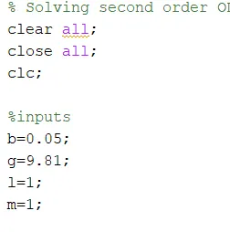
We assign value of b,g,l and m. Here b is damping coefficient, g is gravity, l is length of string of pendulum and m is the mass of bob.
2. Next we assign the time span for we are observing the motion. Initial conditions are defined by us for the position and velocity of bob.
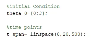
These are the important factors on which the motion of pendulum is defined.
3. This is the most important of our programme. For computing the ODE there is an inbuilt function in MATLAB naming “ode45”.

It takes a function and three data as arguments. The first part of the function is the equation which is going to be integrated. We have input the integrating equation in form of a function named “secondOde”.
The other arguments are the limits in between which the equation is going to be integrated.
The received outputs are two arrays. First array is the time span and the second is the dataset for angular position and velocity.
4. Next we tried to plot the graph of angular velocity and angular position versus time.
For this we first take a variable in which saves the data for angular position and one more variable in which the angular velocity array is saved.
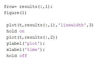
After that plotting is done by using the “plot” command. Labelling of the axes is also done.
Hold on is used to plot the next plot on the same graph. Again hold off is used to make the plot complete otherwise further plotting would also be done on the same figure.
5. Next we move on to describe the motion of th simple pendulum. For this our approach to make the motion visible of the bob with help of plotting consecutive co-ordinates.
We tried to iterate a loop by which it plotted each time different coordinates on the graph.
X-coordinate and T-coordinate is evaluated using simple trigonometry.
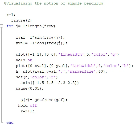
After a new figure is initiated and plotting is done.
We have created a fixed beam on to which bar of pendulum hinged.
The hinged point is the centre of the plot. Towards y axis our pendulum is hanging.
For making the bob we have used the marker command. Basically marker command is used to mark a point on a particular graph but by increasing the size of the marker we have displayed it as a bob.
Range of x and y axes are fixed using axis command. Also a pause of 0.05 Seconds has been created in the loop.
6. Making the Animation:-
For making animation we have saved every output of the loop as a frame in the B array. For this purpose only we have initiated a “r” counter. This r will act as indexing for the array.
Now every data of the loop is saved in the loop as a set of frames which is accomplished by “getframe” command. The only work left is to make them converted into a video file.
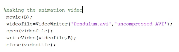
For movie making we have used the given steps starting with movie command which converts every frame of array B into a movie.
So, in this way animation is made to fulfil our purpose.
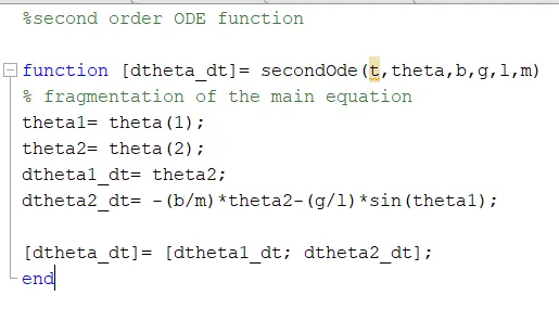
7. We have created a function “secondOde” for writing our differential equation.
`(d^2/dt^2)*θ+(b/m)*(d/dt)*θ+(g/l)*sinθ=0`
By using the mathematical formulations as described in the theory section this function is constructed for solving the equation.
Problems Faced:-
“Problems or errors are the real milestone on the journey of learning.”
These are the evidences that we are enhancing in our subject.
The first issue i have faced was regarding using axis command. I have not placed the axis command at correct position which was resulting in a discomfort view of the plot.
To rectify it I placed before the pause command.
Next issue was showing the two outputs in two different figures. The reason was that i was using only figure to show two different plots . I rectified it using two different figures and using hold on and hold off commands.
The logical section of the programme to describe the motion was really challenging to me. It was appearing pretty difficult for me to create the logic using a mathematical model. For this purpose, I discussed with my mentor for this. By discussing with him I felt the intuition behind this programme and correctly describe the motion of the pendulum.
Results:-
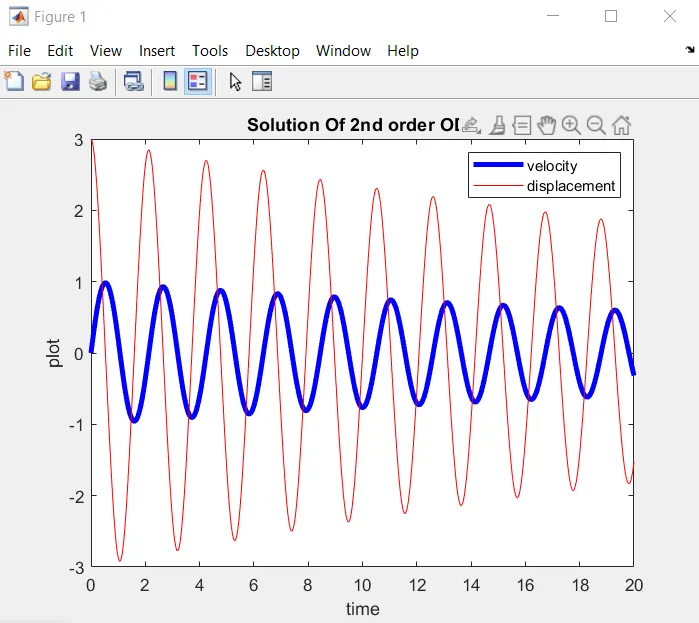
In total there are three final results of our programme. The first one is the graph of position versus time of the bob. Second is the graph of angular velocity of bob versus time.
We have tried to plot the two graphs on same plot.Figure 1
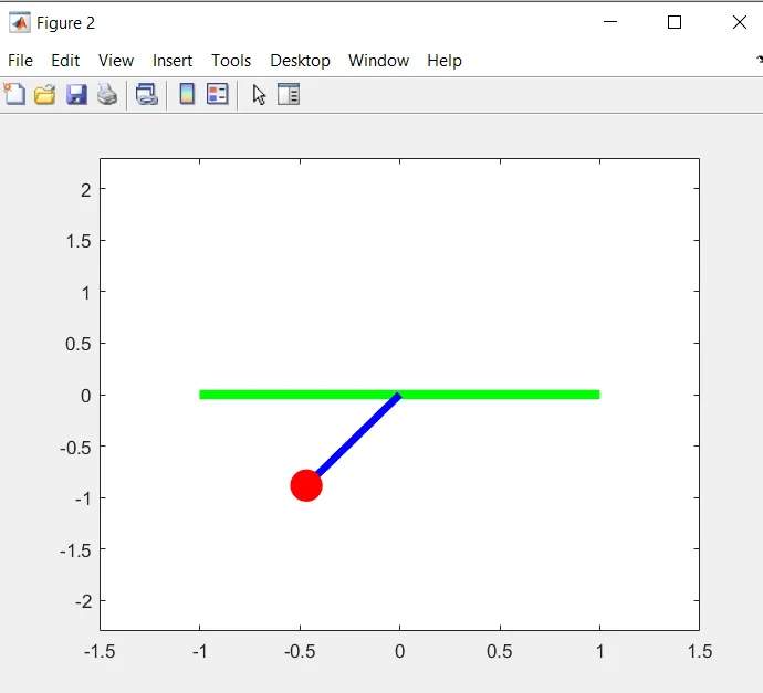
Click here to view the animation
Conclusion:-
I successfully completed the plotting the graph after evaluating all the datasets. Animation is running fluently and giving us a proper decription of the pendulum’s motion.
This project was really bold due to the reason it motivated as well s compelled me to think about logical aspect behind mathematical modelling the matlab programmes.
It introduces me to real matlab application in which we can compute even a complex situation very efficiently.
With the proper guidance of my mentor I am able to finally complete this project in the give time bound.
--------------The End------------
% Solving second order ODE for simple pendulum
clear all;
close all;
clc;

%inputs
b=0.05;
g=9.81;
l=1;
m=1;

%initial Condition
theta_0=[0;3];                     %value of initial position and velocity

%time points
t_span= linspace(0,20,500);        %time span for which motion is going to be obseved

%solve ODE
% use of inbuilt ode45 function
[t,results]= ode45(@(t,theta) secondOde(t,theta,b,g,l,m),t_span,theta_0);

frow= results(:,1);
figure(1)

 plot(t,results(:,1),'linewidth',3,'color','b')
  hold on
 plot(t,results(:,2),'color','r')
 ylabel('plot');
 xlabel('time');
  legend('velocity','displacement')
 title('Solution Of 2nd order ODE')

 hold off


%Visualising the motion of simple pendulum

 r=1;
   figure(2)
 for j= 1:length(frow)

     xval= l*sin(frow(j));
     yval= -l*cos(frow(j));

     plot([-1 1],[0 0],'Linewidth',5,'color','g')
     hold on
     plot([0 xval],[0 yval],'Linewidth',4,'color','b');
     h= plot(xval,yval,'.','markerSize',60);
     set(h,'color','r')
       axis([-1.5 1.5 -2.3 2.3])
     pause(0.05);

       B(r)= getframe(gcf);
      hold off
       r=r+1;

 end

 %Making the animation video
  movie(B);
  videofile=VideoWriter('Pendulum.avi','uncompressed AVI');
  open(videofile);
  writeVideo(videofile,B);
  close(videofile);
%second order ODE function

function [dtheta_dt]= secondOde(t,theta,b,g,l,m)
% fragmentation of the main equation
theta1= theta(1);
theta2= theta(2);
dtheta1_dt= theta2;
dtheta2_dt= -(b/m)*theta2-(g/l)*sin(theta1);

[dtheta_dt]= [dtheta1_dt; dtheta2_dt];
end