RANKINE CYCLE SIMULATOR

AIM:-

To programme a Rankine cycle simulator

OBJECTIVE:-

We have been provided with a pre programmed function naming "XSteam.m". This function is designed to calculate values of steam table.

In this project we have to programme rankine cycle simulator win MATLAB with using the given function.

The motive is to find the net output workk and plot the graphs of t vs s and h vs s. We have to also display different state properties in command window. Here the pressure and temperatureat turbine inlet will given as input alongwith the turbine outlet pressure.

THEORY:

Rankine cycle is a theoretical vapour power cycle on which steam turbines work.

It comprises of four different paths on which the thermodynamic processes undergo.

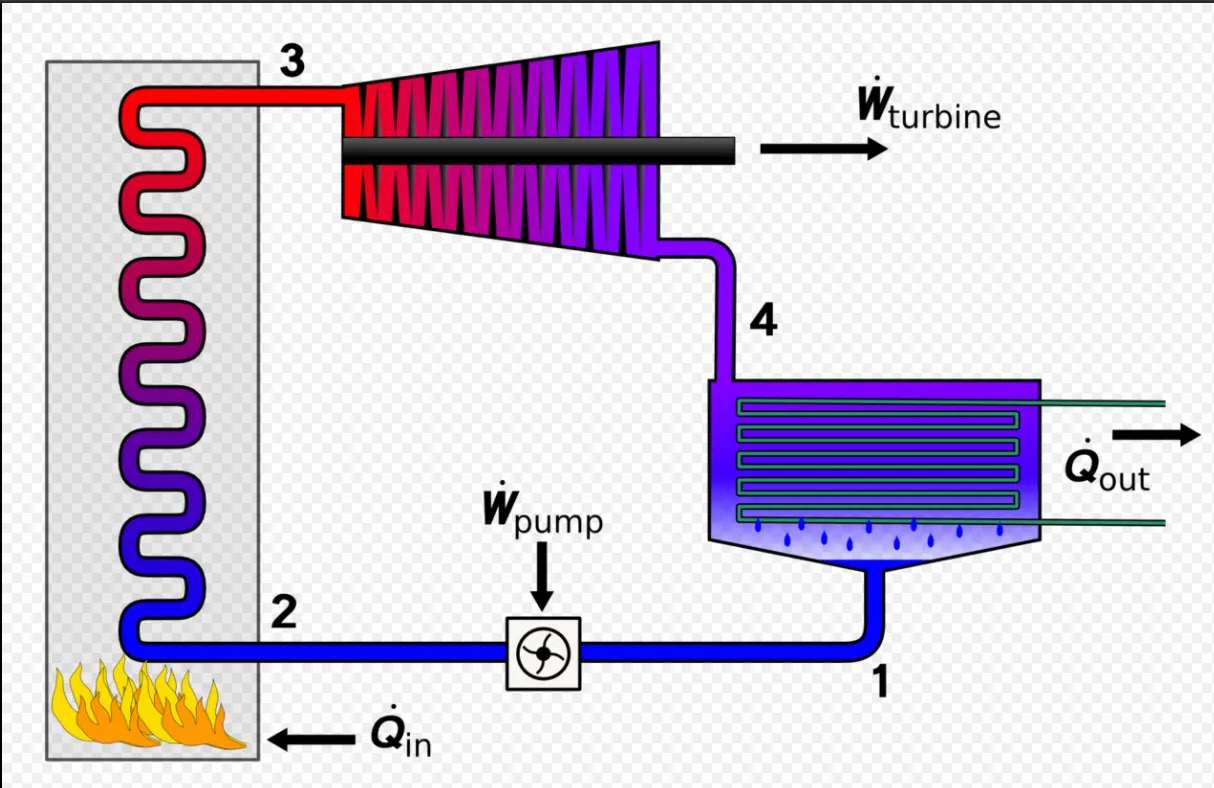
The rankine cycle has four basic units which are:-

• Turbine
• Condenser
• Pump/compressor
• Boiler

We will be discussing all the process with the given as reference.

1. Process 1-2 is an isentropic process. In this process the steam goes in a reversible adiabatic expansion. Moreover, during this process the entropy of the system remains constant.

The steam coming from the boiler does a positive work on turbines which provides it a rotational motion. From this rotational motion various mechanical and electrical works are accomplished. Due the positive work on turbines in a adiabatic process the steam lowers it temperature.

After this the steam enters to the condenser.

2. Process 2-3 is an isobaric process. During this process the heat is lost by the gas to the condenser. This process is a very crucial step because in this step the gas is converted into liquid which is then pumped by hr pump to boiler. Basically condensation of the gas takes place in this step.

3. Process 3-4 is again an isentropic process. In this process the liquid goes an adiabatic expansion. From this process the liquids is pumped to boiler for further process.

4. Process 4-1 is isobaric process. Here the liquid is converted into steam at temperature and pressure. This steam then follows the further cycle.

For finding values of different state properties, steam table is used. With the help of steam table we will be able to find the enthalpy and entropy of the system at different points.

Here work is done in only two processes. These are in the turbine and other one is in the pump.

We will be using steady flow equation for finding work done at the two stages.

`Q-w=gradH`

For the work done in turbine (Wt)

`W=h1-h2`

Likewise, work done by pump is

Wp=h4-h3

We know from basic thermodynamic principles efficiency is defined as the ratio of net work done by the system to total heat supplied.

Moreover, heat is supplied only in boiler and value will be

H1-h4.

Therefore, thermal Efficiency will be written as :

`n=((h1-h2)-(h3-h4))/(h1-h4)`

Next is the back work ratio which is defined as the fraction of the work produced by the turbine that is consumed by the compressor.

`BWR=(h4-h1)/(h1-h2)`

S.S.C is the acronym of specific steam consumption which is defined as the net steam consumed by the cycle per unit power output.

Mathematclly, it can be written as

`S.S.C= 3600/text(Wnet)`

Procedure:

The whole programming process includes--

• finding the state points
• displaying each result
• plotting the graphs

Steps for each of this process have described sequentially.

In place of steam table we will be using the “XSteam” function which is provided to us.

1. First we will find the state points of the rankine cycle which include entropy, enthalpy, temperatures and pressure.

For this process, we will follow the techniques as discussed in theory part.

Initial state temperature and pressure will be inputted by us.

We begin with point 1; here first of all we will find h1 with help of steam table.

Likewise s1 will be found out.

Next for state 2,

s2= s1

and by using the eqn,

s2= sf + x*sfg

x will be found and use to determine h2.

Values of hf ,sf,hfg,sfg will be taken from XSteam function by using proper arguments as shown in the code.

Moving on further we will compute h4,s4 ,s5,s6. The theoretical aspect has been clearly discussed previously here all the codes has been shown on how to execute it.

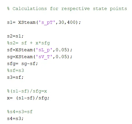
So, by end of this step we will have our all state datas and now we can move on plotting the points.

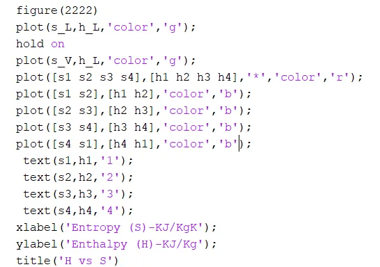
2. We begin plotting by first plotting the saturated vapour and liquid curves for this we will have to first calculate the entropy and enthalpy for saturated conditions. Help of a loop has been taken for this purpose.

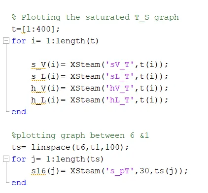
Figure has been started inside which t vs s will be plotted.

All the path lines have been plotted along with state points with help of plot command. Appropriate labels and legends are also mentioned.

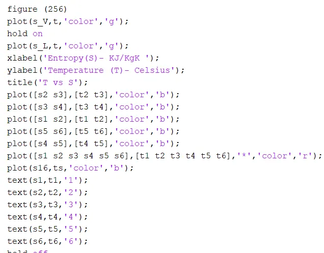
Like wise for fig 2 all works have been done and yhe code is executed.

For labelling the state number text command has been used.

3. Next the only job left is displaying the computed results.

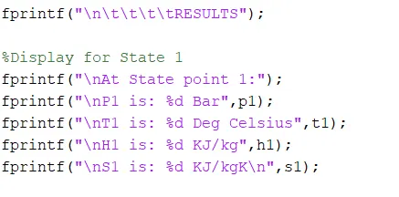
So all the results have been displayed in the command window using the “fprintf” command. Below we have snap of first state points displaying as same will be repeated for rest of the points.

RESULTS:-

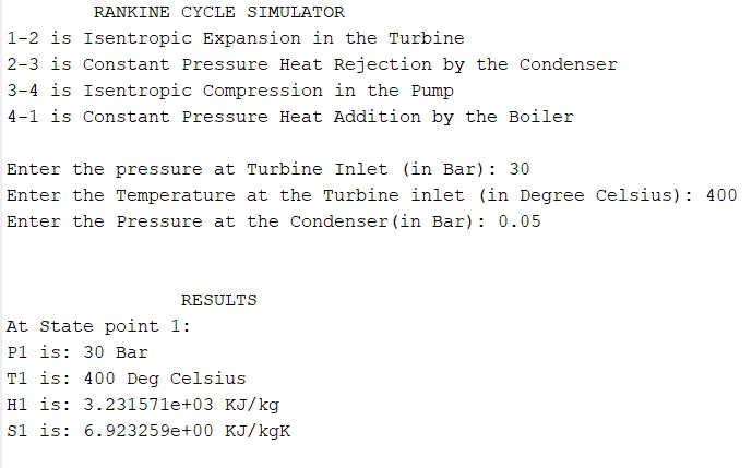
In the final output we will have to show the command window and the two plots.

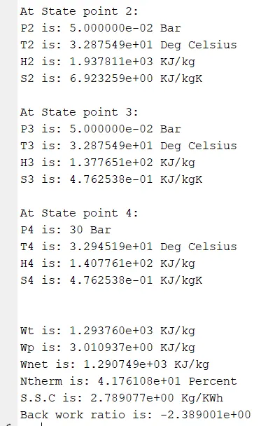
1. In the command window values of all the state properties alongwith the properties of every path has been shown.

2. In the graphs T vs H and H vs s has been plotted . By this graphs we are getting the intuition how the rankine cycle is progessing at every step.

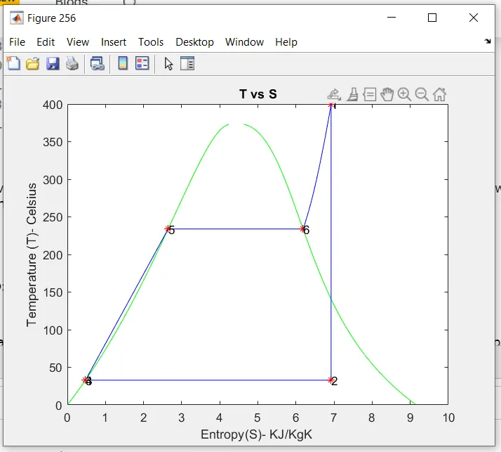
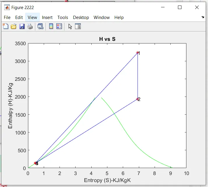
So we get net output work as 1290.7 kj/kg

back work ratio= -2.38

CHALLENGES FACED:-

1. First problem I faced was just a simple coding error in which by mistake I had used different loop counter as was assigned the loop code.

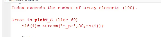
2. A major challenge that is faced by me and expected to be faced by every person that solve this project understands the “XSteam” function.

It found me pretty good amount of time to analyse how to use the given function. If one has found the way to efficiently use the function then the person can easily solve the rest of the project.

CONCLUSION:-

I got a very useful lesson in solving complex programming questions that is “PATIENCE”.

This report made me able to pounder sequentially on robust questions. It instigates me to do a little more effort to solve this challenge.

At last, I want to say this was one of finest MATLAB project I have ever made.

REFERENCES:-

1. Engineering thermodynamics by P.K Nag

2. Fprintf documentation --https://www.mathworks.com/help/matlab/ref/fprintf.html

CODE of the programme:-

%Programme of RANKINE CYCLE SIMULAOR
close all;
clear all;
clc;


%Path properties
fprintf("ttRANKINE CYCLE SIMULATOR");
fprintf("n1-2 is Isentropic Expansion in the Turbine");
fprintf("n2-3 is Constant Pressure Heat Rejection by the Condenser");
fprintf("n3-4 is Isentropic Compression in the Pump");
fprintf("n4-1 is Constant Pressure Heat Addition by the Boilern");

%Giving inputs for the initial conditions
p1= input("nEnter the pressure at Turbine Inlet (in Bar): ");
t1= input("Enter the Temperature at the Turbine inlet (in Degree Celsius): ");
p2= input("Enter the Pressure at the Condenser(in Bar): ");
fprintf("n");
%p1= 30;
p4=p1;
%p2= 0.05;
p3=p2;

% Calculations for respective state points

s1= XSteam('s_pT',30,400);

s2=s1;
%s2= sf + x*sfg
sf=XSteam('sL_p',0.05);
sg=XSteam('sV_T',0.05);
sfg= sg-sf;
%sf=s3
s3=sf;

%(s1-sf)/sfg=x
x= (s1-sf)/sfg;

%s4=s3=sf
s4=s3;

s6= XSteam('sV_p',30);
s5= XSteam('sL_p',30);

%T_ps	Temperture as a function of pressure and entropy
%t1=400;
t2= XSteam('T_ps',0.05,s2);
t3=t2;
t4= XSteam('T_ps',30,s4);
t5= XSteam('T_ps',30,s5);
t6= XSteam('T_ps',30,s6);

%Calculations of H
h1= XSteam('h_pT',30,400);


%h2= hf + x*hfg
hf= XSteam('hL_p',.05);
hg= XSteam('hV_p',0.05);
hfg= hg - hf;

h2= hf + (x*hfg);

h3= hf;

% V3*(p4-p3)= (h4*h3);

v3= XSteam('vL_p',0.05);
h4 = (( v3 * (p4-p3)*10^5)/10^3) + h3;



%Calculation of efficiency and work done at different stages

Wtur= h1-h2;               %work done by turbine
Wpump= h4-h3;              %work done by pump
Qin= h1 - h4;              %heat given to the cycle
Wnet= Wtur - Wpump;        %Net work done
Ntherm= Wnet/Qin;          %Thermal Efficiency
steamRate= 3600/(Wnet);    %Specific Steam Consumption
BWR=(h4-h1)/(h1-h2);       %Back work ratio



% Plotting the saturated T_S graph
t=[1:400];
for i= 1:length(t)
    
    s_V(i)= XSteam('sV_T',t(i));
    s_L(i)= XSteam('sL_T',t(i));
    h_V(i)= XSteam('hV_T',t(i));
    h_L(i)= XSteam('hL_T',t(i));
end

%plotting graph between 6 &1
ts= linspace(t6,t1,100);
for j= 1:length(ts)
    s16(j)= XSteam('s_pT',30,ts(j));
end



%Displaying the results in command window
fprintf("nttttRESULTS");

%Display for State 1
fprintf("nAt State point 1:");
fprintf("nP1 is: %d Bar",p1);
fprintf("nT1 is: %d Deg Celsius",t1);
fprintf("nH1 is: %d KJ/kg",h1);
fprintf("nS1 is: %d KJ/kgKn",s1);


%Display for state 2

fprintf("nAt State point 2:");
fprintf("nP2 is: %d Bar",p2);
fprintf("nT2 is: %d Deg Celsius",t2);
fprintf("nH2 is: %d KJ/kg",h2);
fprintf("nS2 is: %d KJ/kgKn",s2);

%Display for state 3

fprintf("nAt State point 3:");
fprintf("nP3 is: %d Bar",p3);
fprintf("nT3 is: %d Deg Celsius",t3);
fprintf("nH3 is: %d KJ/kg",h3);
fprintf("nS3 is: %d KJ/kgKn",s3);

%Display for State 4
fprintf("nAt State point 4:");
fprintf("nP4 is: %d Bar",p4);
fprintf("nT4 is: %d Deg Celsius",t4);
fprintf("nH4 is: %d KJ/kg",h4);
fprintf("nS4 is: %d KJ/kgKn",s4);

%Display for properties of whole cycle
fprintf("nnWt is: %d KJ/kg",Wtur);
fprintf("nWp is: %d KJ/kg",Wpump);
fprintf("nWnet is: %d KJ/kg",Wnet);
fprintf("nNtherm is: %d Percent ",Ntherm*100);
fprintf("nS.S.C is: %d Kg/KWh",steamRate);
fprintf("nBack work ratio is: %d ",BWR);
fprintf("n");

%plotting the t vs s curve  
  figure (256)
  plot(s_V,t,'color','g');
  hold on
  plot(s_L,t,'color','g');
  xlabel('Entropy(S)- KJ/KgK ');
  ylabel('Temperature (T)- Celsius');
  title('T vs S');
  plot([s2 s3],[t2 t3],'color','b');
  plot([s3 s4],[t3 t4],'color','b');
  plot([s1 s2],[t1 t2],'color','b');
  plot([s5 s6],[t5 t6],'color','b');
  plot([s4 s5],[t4 t5],'color','b');
  plot([s1 s2 s3 s4 s5 s6],[t1 t2 t3 t4 t5 t6],'*','color','r');
  plot(s16,ts,'color','b');
  text(s1,t1,'1');
  text(s2,t2,'2');
  text(s3,t3,'3');
  text(s4,t4,'4');
  text(s5,t5,'5');
  text(s6,t6,'6');
  hold off

  
  %plotting the h vs s curve 
 figure(2222)
 plot(s_L,h_L,'color','g');
 hold on
 plot(s_V,h_L,'color','g');
 plot([s1 s2 s3 s4],[h1 h2 h3 h4],'*','color','r');
 plot([s1 s2],[h1 h2],'color','b');
 plot([s2 s3],[h2 h3],'color','b');
 plot([s3 s4],[h3 h4],'color','b');
 plot([s4 s1],[h4 h1],'color','b');
  text(s1,h1,'1');
  text(s2,h2,'2');
  text(s3,h3,'3');
  text(s4,h4,'4');
 xlabel('Entropy (S)-KJ/KgK');
 ylabel('Enthalpy (H)-KJ/Kg');
 title('H vs S')

X----------------The End----------------X