Air stranded Cycle
Aim:-
Write code To Plot the P-V graph of air stranded Otto Cycle.
Objectives:-
A running situation of air stranded cycle is given to us. In thermodynamical aspect this cycle is called The Otto Cycle.
In this project, we are provided with the engine specifications of a SI Engine. We are provided with the bore, compression ratio, length of connecting rod and isentropic constant (gamma) of atmospheric air.
Point 1 is the starting point of the process and we are provided with the initial Temperature and Pressure.
The process is going through a 4 state points, namely 2,3 and 4. We have to evaluate pressure and temperature at all these three remaining points.
Moreover, we have to also find the thermal efficiency of the provided Otto cycle. These whole processes which include plotting of graphs and mathematical calculations are going to be done on Matlab using codes.
After finding the state variables at each position, we have to plot the graph of the Otto cycle. For this we have to clearly show which path is being followed by the air for completing the process.
Theory:-
Air stranded cycle is term given to the thermo-dynamical cycle in which working medium is considered to be air. Otto cycle is a specific air stranded cycle used in the petrol, gas or other fuel engines.
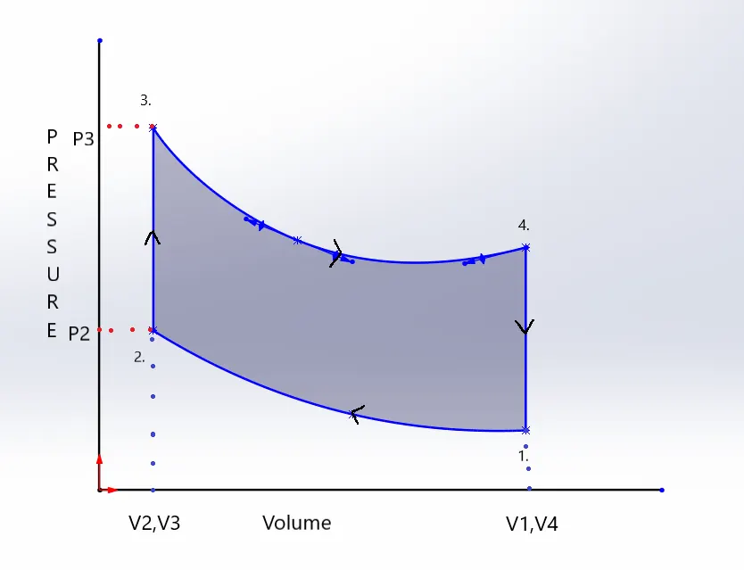
We have taken 1 as the starting point of the cycle. The air is going from 1 to 2 then 2 to 3 and 3 to 4, finally reaching to 1.
The specifications of engine are provided to us which include bore, length of connecting rod, compression ratio, stroke length.
Compression ratio is given to us and we have taken it as “r”. Compression ratio is defined as ratio of maximum volume to minimum volume in the cylinder. Maximum volume inside the cylinder will be sum of clearance volume and swept volume ie.
Vmax= Vc + Vs
Minimum volume inside the cylinder will be the clearance volume.
Vmin= Vc
Therefore from definition the compression ratio will be expressed as:-
`r= (Vmax)/(Vmin)`
From plot of our cycle it can be expressed as:-
`r= (V1)/(V2)=(V4)/(V3)`
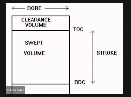
Calculation of Swept volume:-
Piston covers an area equivalent to a cylinder having length equals to stroke length and radius equal to half the bore. Equation to calculate swept volume can be written as:-
`Vs=(π/4)*(b o re)^2*stroke`
Calculation of clearance volume:-
With the help of compression ratio clearance volume can be calculated easily as
`Vc= (Vs)/(r-1)`
From analysing the graph, it has been cleared that V1 and V4 are maximum volumes and V2 and V3 are minimum volumes. Therefore in other words, it can be said that:-
`Vmax=V1=V4`
`Vmin=V2=V3`
Now the volume of V1= Vc+Vs And V2=Vc.
Characteristics of each path have been briefly explained.
Process 1 -2
Process going from 1 to 2 is an isentropic constant. In this process an adiabatic and reversible compression of the air is done by the system.
Since the working medium is air we take gamma as 1.4.
We are provided with the P1,V1 and T1 we can find P2 and T2 by using the equations of adiabatic processes as 1-2 is an isentropic process.
`(P1)/(P2)=((V1)/(V2))^γ`
`P2=P1*r^γ`
Now we have the value of P2, V2. By using universal gas equation T2 can be calculated as
`T2= (P2*V2*T1)/(P1*V1)`
Process 2-3
This process is an isochoric expansion of gas. In this case the expansion of gas is done by increasing the pressure at a constant volume.
Since this process is isochoric therefore V2=V3.
Temperature at Point 3 is also known to us and we will denote it by T3.
For pressure at point 3
By using Gay Lussac’s law we can say
`(P3)/(T3)=(P2)/(T2)`
Therefore,
`P3=T3* (P2)/(T2)`
Process 3-4
In this process gas is undergoing an isentropic expansion. It means this is process of adiabatic and reversible expansion.
Since it is an adiabatic process and volume at point 4 is known to us we can find P4 as
`(P3)/(P4)=((V4)/(V3))^γ`
Therefore,
`P4=P3*((V3)/(V4))^γ`
`P4=P3*(1/r)^γ`
Process 4-1
In this case the air is going isochoric compression.
By using Gay Lussac’s law T4 can be evaluated.
`T4=P4* (T1)/(P1)`
Hence by doing all the mentioned points we can easily compute the state variables namely pressure, volume and temperature at each point.
Calculations of V at random points in isentropic curves:-
We have used this formula for our purpose:-
`V/Vc=1+(1/2)*(cr-1)*[R+1-cosθ-(R^2-(sinθ)^2 )]`
Where theta is the angle between connecting rod and vertical.
Calculation of thermal efficiency:-
Thermal efficiency of any thermodynamic cycle is defined as the ratio of net work done and total heat supplied to the system.
Work done = Heat supplied – heat rejected
Process in which heat supplied is 3 -4.
Process in which heat is rejected is 1-2.
Therefore,
Heat Supplied= mCv(t2-t3)
Heat rejected= mCv(t4-t1)
Thermal Efficiency= (Heat supplied-heat rejected)/heat supplied
After putting appropriate values we get,
Thermal Efficiency= `(1-((t2)/(t1)) )`
Code:-
- Our code starts from clearing the command line, closing all running applications and clearing all the saved workspace data.
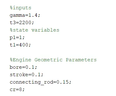
2. Second comes the inserting available data. We have available with us the engine specifications. We specify the bore, stroke and other parameters by storing them in different variables.
Also we assign the initial temperature and pressure by storing them in t1 and p1 respectively.
3. Now, we will proceed to do our first calculations of finding maximum and minimum cylinder volume.
Maximum volume will be the sum of clearance and swept volume. Minimum volume will be the clearance volume.
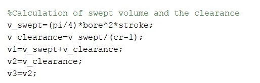
Maximum volume and minimum volume portraits the v1 and v2 of the graph respectively.
4. Moving on further, we will evaluate state variables at each point.
For pressure and temperature at point 2:
Process 1-2 is a isentropic process, therefore pressure and volumes can easily be calculated as shown below.
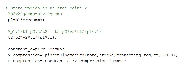
Regarding the plotting points between 1 and 2, we have used the function “pistonKinematics”. Details about this function are briefly explained further in this report.
5. After the calculation of pressure and temperature at point 2, we will proceed towards point 3.
Since process 2-3 is an isochoric process volume of gas at points 2 and 3 will remain constant. We know the value of temperature at 3; therefore P can easily be calculated by using Universal Gas Equation as shown in theory section.
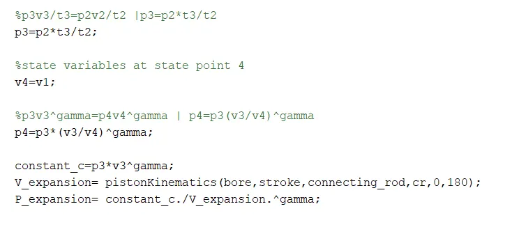
6. Process 3-4 is an isentropic expansion. Also, volume of gas is known to us which is equal to volume of gas at point 1.
Therefore, volume and temperature at point 4 can easily be evaluated by using equations of adiabatic process; the same is done by the codes.
7. Now we move on plotting of graph. Process 2-3 and process 4-1 are isochoric, so there path can easily be drawn by using straight lines.
We will have to do some extra efforts in plotting graph of the two isentropic processes. For this we have used a function named as “pistonKinematics”.
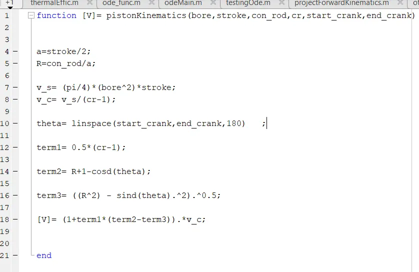
We have defined the function with six arguments. Output will be a array. The motto behind using this function is to find the volume inside the cylinder at numerous values. By using this various values of volumes we will find the corresponding values of pressure.
The concept behind this has already been explained. The whole equation is fragmented into three parts to simplify our calculations.
The first part is 0.5* (cr-1)
Second part is R+1-cosd(theta), cosd() is used because the angle input will be in degrees.
Third and the last part is (R^2- sind(theta)^2)^0.5
Finally these three terms are arranged to get our final result.
8. For thermal efficiency calculation we have again used a function naming “thermaEffic”.
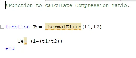
It takes two arguments t1 and t2 and give output is Te.
The output is the thermal efficiency of the Otto cycle.
9. Finally we have done the plotting by using different data sets.
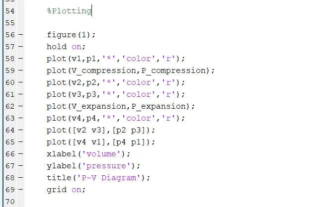
First we plot the co-ordinates of pressure and volumes of points 1, 2, 3 and 4 using the plot commands.
After that we plot the straight lines for 2-3 and 4-1. And curves for 1-2 and 3-4. A suitable colour is assigned to the curves as well as lines.
Xlabel and ylabel commands are used to name the axes. A suitable title is given to the plot using title command. We have also put on the grids on.
Results:-
Our final outcomes of this project are the coordinates of the four given points on P-V graph and a P-V graph. Along with this thermal efficiency has also been calculated.
Underlying is the plot which is created by above given processes.
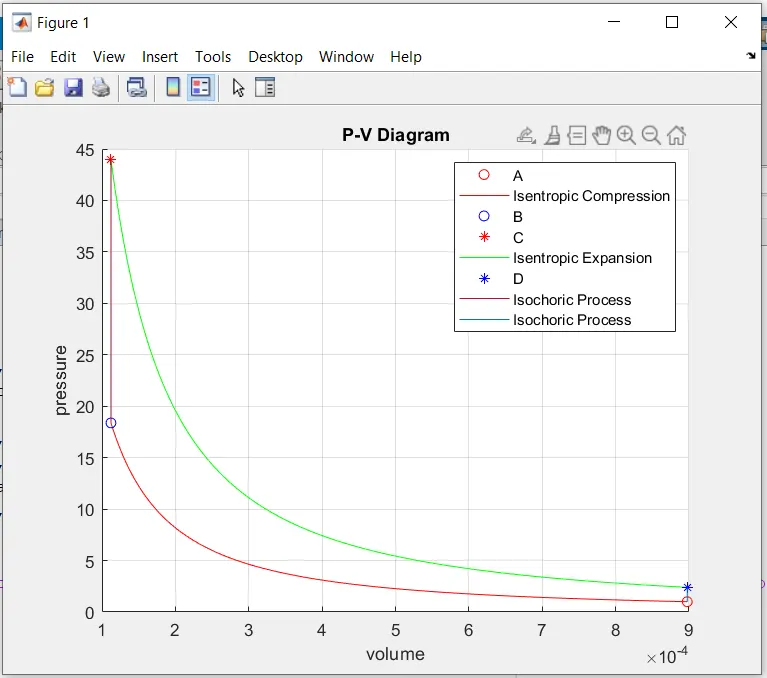
The result is scripting how pressure and volume is changing in the cylinder with the progress of the cycle. Area of the curve will give us the work done by the gas.
In command window we received the value thermal efficiency.
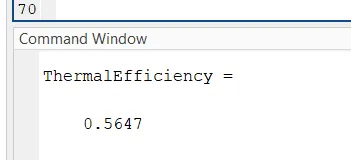
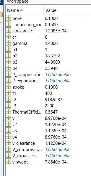
So, in total there are three given sets of output coordinates of the four points, P-V graph and thermal efficiency. Underlying is the snap of workspace after the programme has been run.
Errors faced:-
- I got an error in choosing a variable to store output of the given function. The error was that I have used space in variable name which is wrong according to matlab programming.
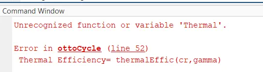
I rectified by eliminating the space between the names.
2. Here I have used hash for plotting the coordinates which is wrong from matlab programming point of view. Hash has a inbuilt meaning in matlab library, therefore it shown an error.
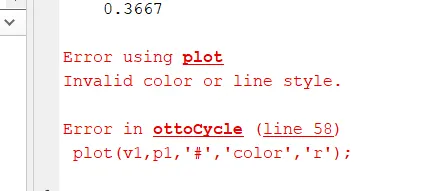
I rectified by using “*” in place of “#”. We can use any other symbol also.
3. This error is shown because I have used clear all, close all and clc in the function programme file of thermaleffic function.
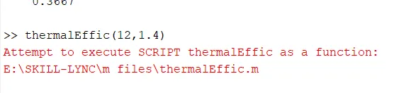
I have rectified it by erasing all those three commands. After that my programme started to run properly.
Conclusion:-
In this project I have used MATLAB programming to solve an OTTO cycle. Initial temperature and pressure was given to me. Along with that engine specification was also provided to me.
It takes me to create two additional functions in order to make my programme run efficiently.
The final result of the programme was a P-V plot and value of thermal efficiency.
Several errors were confronted by me during the span of coding the programme. But with proper concepts I tried to figure out the errors.
In this report, all the theoretical aspect and procedure of the programming is serially mentioned. I tried my best to clear every concept and endeavoured to sublime every doubt of the readers.
% Programme to evaluate an Air stranded cycle
% Calculation in Otto Cycle
clear all;
close all;
clc;

%inputs
gamma=1.4;
t3=2200;
%state variables
p1=1;
t1=400;

%Engine Geometric Parameters
bore=0.1;
stroke=0.1;
connecting_rod=0.15;
cr=8;

%Calculation of swept volume and the clearance
v_swept=(pi/4)*bore^2*stroke;
v_clearance=v_swept/(cr-1);
v1=v_swept+v_clearance;
v2=v_clearance;
v3=v2;

% State variables at stae point 2
 %p2v2^gamma=p1v1^gamma
 p2=p1*cr^gamma;

 %p1v1/t1=p2v2/t2 | t2=p2*v2*t1/(p1*v1)
 t2=p2*v2*t1/(p1*v1);

 constant_c=p1*v1^gamma;
 V_compression= pistonKinematics(bore,stroke,connecting_rod,cr,180,0);
 P_compression= constant_c./V_compression.^gamma;

 %p3v3/t3=p2v2/t2 |p3=p2*t3/t2
 p3=p2*t3/t2;

 %state variables at state point 4
 v4=v1;

 %p3v3^gamma=p4v4^gamma | p4=p3(v3/v4)^gamma
 p4=p3*(v3/v4)^gamma;

 constant_c=p3*v3^gamma;
 V_expansion= pistonKinematics(bore,stroke,connecting_rod,cr,0,180);
 P_expansion= constant_c./V_expansion.^gamma;


 %thermal Efficiency
 ThermalEfficiency= thermalEffic(t1,t2)

 %Plotting

 figure(1);
 hold on;
 plot(v1,p1,'o','color','r');
 plot(V_compression,P_compression,'color','r');

 plot(v2,p2,'o','color','b');
 plot(v3,p3,'*','color','r');
 plot(V_expansion,P_expansion,'color','g');
 plot(v4,p4,'*','color','b');
 plot([v2 v3],[p2 p3]);
 plot([v4 v1],[p4 p1]);
  legend('A','Isentropic Compression','B','C','Isentropic Expansion','D','Isochoric Process','Isochoric Process');
 xlabel('volume');
 ylabel('pressure');
 title('P-V Diagram');
 grid on;
%function to claculate coordinates of PV curve in isentropic process
function [V]= pistonKinematics(bore,stroke,con_rod,cr,start_crank,end_crank)


a=stroke/2;
R=con_rod/a;

v_s= (pi/4)*(bore^2)*stroke;
v_c= v_s/(cr-1);

theta= linspace(start_crank,end_crank,180)   ;

term1= 0.5*(cr-1);

term2= R+1-cosd(theta);

term3= ((R^2) - sind(theta).^2).^0.5;

[V]= (1+term1*(term2-term3)).*v_c;


end
%Function to calculate Thermal Efficiency.
function Te= thermalEfiic(t1,t2)
Te= (1-(t1/t2))
end