CURVE FITTING

AIM:-

• Write code to fit a linear and cubic polynomial for the Cp data.
• Plot the linear and cubic fit curves along with the raw data points.

OBJECTIVE:-

In this project we are going to do theoretical study and programming analysis on curve fitting.

We have been provided with a dataset of temperature versus CP of particular substance.

We have to find out a suitable linear ad cubic curve corresponding to the given raw dataset.

Moreover, we have to do analysis on how to properly fit a curve corresponding to given datasets.

THEORY:-

We are doing regression analysis of a given dataset to find a suitable curve for it.

Curve fitting

The process of finding an appropriate curve for a given dataset to fit the curve most optimally is known as curve fitting.

We are focused on doing our estimations on polynomial curve.

On the fitness level of the curve the degree of the polynomial is increased or decreased. To ensure the proper fitness of a curve various methods can be adopted. We will be using the R-square method as this is a most efficient and easiest way.

Curve fitting process is a mathematical toolbox which used a simulative algorithm to find the coefficients of the assumed polynomial.

Finding the coefficients

Let us visualise a situation in which a set of dataset is provided to us. We have found a proper curve for fit.

To start with the formulation we will assume a polynomial function. Let our polynomial equation be

`f(x)=A1+A2*x^2+A3*x^3+⋯+An*x^n`

We will calculate the value of polynomial at every x coordinates. Let them be f(xi).

The original data be Y(i). Now error at every point will be calculated.

Error= `| Y(i)-f(x i) |`

For removal of modulus, we will prefer squaring of the individual errors.

In this way Sum of squared errors will be evaluated

`SSE= ∑_(i=1)^n(error(i))^2`

Now for finding polynomial coefficients SSE will be differentiated individually by each of A1, A2 and so on and equated to zero.

`[((∂SSE)/(∂A1)),((∂SSE)/(∂A2)),((∂SSE)/(∂A3)),(…..),((∂SSE)/(∂An))]= 0`

After solving of the above equation we will get our coefficients of the polynomial equation.

This whole process of finding the equation for a given dataset is called as Least Square Method(LSD).

Now we will proceed to check the fitness of the curve by R square method.

R-square Method

First we will find the mean of the given dataset. Let us represent it by M.

After that SSR will be evaluated as follows:-

`SSR=∑_(i=1)^n(f(x(i)+Mean)^2`

Now,

SST= SSE+ SSR

`R^2=(SSE)/(SST)`

In this way R-squared will be evaluated by the given algorithm.

The value of R-square lies between zeros to one. Greater the value of R-square the more perfect the fit.

CODE:-

Code for cubic polynomial for cp data

1. First we will initiate our coding by giving the initial three commands that will close all the running matlab programs, clear the command window and clear the workspace.

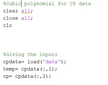
After that we will load the given dataset in our programme by using “load” command.

Temperature column of the data and cp column will be differentiated in two different arrays.

2. Next we will find the coefficient of our assumed polynomial equation.

In this equation we have assumed it to be a cubic polynomial, so our assumed equation will be

`f(x)=a*x^3+b*x^2+c*x+d`

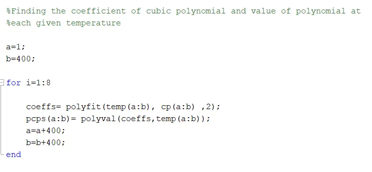
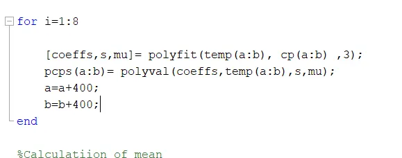
Here to optimise our curve fitting process the concept of splitting of curve has been used. Applying this we have splitted the whole dataset into eight parts. Now we will have to find eight different polynomials and have to find coefficients of all the eight equations.

For accomplishing this job we have taken help of loop. We have iterated to eight times for finding the required coefficients.

The coefficient are used to generate the polynomials and finding the predicted cps data which are the stored in “pcps” array.

In this way our curve is generated, now the only work left is checking the fitness of the curve.

3. Checking the fitness of the curve

We will be opting the R-square method for measuring the curve fitness.

First the mean of the given data will be calculated.

For mean calculations we have taken help of loop as mentioned in the snap below.

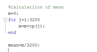
4. Next we move on the calculation of sum of squared errors. It means square of every individual at every temperature co-ordinates.

For this purpose also, we have used the loop.

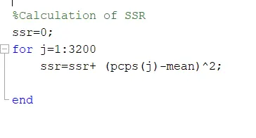
Finally we have calculated the value of R-square by applying the formula:-

`R^2=(SSE)/(SSR+SSE)`

The values of R-square will determine the fitness of the curve.

Code of linear polynomial for CP data

This whole programme will be built in the same manner as the programme for cubic polynomial is made.

1. Starting from losing all the running programs and clearing the command window and loading the given data.

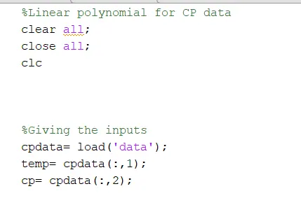
2. After that the ‘polyfit’ and ‘polyval’ operations will be done but as in the cubic polynomial case ewe have splitted the whole dataset into eight parts here in linear case we will be splitting the data in sixteen parts for better curve fitness.

3. This time our assumed equation will be of the form

`f(x)=A1*x+A2`

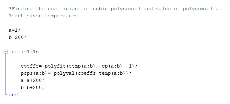
4. Now we will move on checking the fitness of the curve ah=gain bu R-square method.

5. For mean calculation following is done

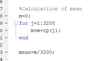
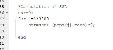
6. Further SSE and SSR are calculated and used for evaluating value of R-square

Code for plotting the curves

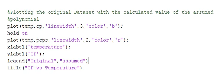
For plotting part in both programmes the codes will remain same. We have first plotted the curve of given dataset and then plotted the curve created by using the data achieved by our assumed polynomial.

For plotting the original and predicted CP values different colors have been used for proper differentiation.

PROBLEMS FACED

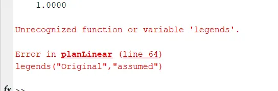
1. First problem I faced was in using the “legend” command. And it was solved by just correcting the spelling.

2. Centring and Scaling

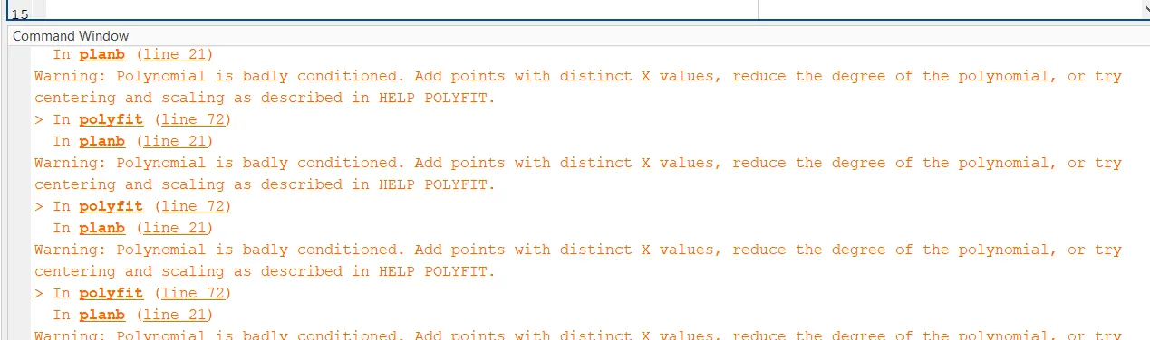
The curve was very constrained in the curve fitting which was appearing as a warning in the command window.

To resolve this I have implemented Centring and scaling method.

This method is used when there is not a proper variation in data. There comes a huge variation in plotting them in terms of scaling on the axes.

So, in process of scaling variables are measured in different units, data are scales to give each variable equal chance to effect the mathematical model.

In this process use of Standard Variation comes into play. The important condition around which this whole process revolves around is that variance of the data distribution is fixed to be unity.

Two parameters are added to the predicted cp and predicting coefficients attribute.

S and mu are added where s is a structure comprissing of three parameters namely :

R ---Triangular factor

Normr---Norm of the residents

`P=(RInv*RInv^' )*(no,rm^2)/(df)`

Where df---Degree of freedom

Next one the mu comprises of two columns . Where mu(1) contains mean and mu(2) contains standard deviation of the dataset,

By using these and the concepts of standard deviation standard variance is scaled to be unity and an optimal curve is granted to us which are evident from the warning removal from the command window.

RESULTS:-

1. In this project there were two parts first one was of cubic polynomial and another was of linear polynomial according to which there are two output plots.

Our first plot will be of cubic polynomial curve. In this plot first the curve is plotted according to the given dataset. Next curve is of value obtained from the assumed polynomial.

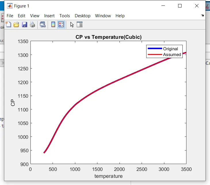
To differentiate between original and assumed, different colours of the curves have been chosen.

2. Next is the plot for the linear polynomial having properties same as cubic.

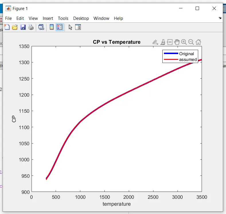
• Due to Value of R-square closer to 1 in both the cases our assumed polynomial has given value very much nearer to original dataset which is making it difficult for us to differentiate between them.
• With the help of Centring and plotting and Least Square Method this curve fit problem has been solved.

DISCUSSION:-

Q. How to make a curve fit perfectly?

Ans.- To make a curve fit we will have to do rigororous regression to eliminate all errors. A perfect fit curve has zero erroe at each and every co-ordinte. To achiev this various splitting can be done or order of the polynomial can be increased.

A perfect fit can be the best fit but a best fit can not be the perfect fit, due to this reason error estimation become a crucial part in curve fitting.

Q. How to get the best fit?

Ans.- For having best fit the error of the curve will have to be minimised. Best fit is that curve which staisfies the given dataset most appropriately. For error estimation vatious methods can be used such as R-square method and many more. In R-square method value of R-square will determine the fitness of the curve. Value of R-square closer to one give a curve very much nearer to the perfection.

Q. What could be done to improve the cubic fit?

Ans.- For improving the cubic curve centering and scaling is come into use. This was done in addition to splitting of the dataset for piecewise analysis. By appropriate scaling down the data the uneven data variation is homogenised. By using the bad condition of our curve was simplified and an optimal polynomial is provided to us.

CONCLUSION:-

This was one of a very logical and pretty project for me.

I got stuck at various places during the interval of programming. It would have been difficult for me my mentor had not supported me. With high concentration and diligence I make this project to come to an efficient conclusion.

By this project, my concepts regarding curve fit have become pretty much clear. I came closer to different applications of MATLAB. I got to know about the concepts of Data Analytics.

I would feel very enthusiasts in doing such projects further more.

MATLAB code for cubic polynomial curve fitting

%Cubic polynomial for CP data
clear all;
close all;
clc



%Giving the inputs
cpdata= load('data');temp= cpdata(:,1);
cp= cpdata(:,2);

%Finding the coefficient of cubic polynomial and value of polynomial at
%each given temperature

a=1;
b=400;

for i=1:8
   
    [coeffs,s,mu]= polyfit(temp(a:b), cp(a:b) ,3);  % Centering And scaling
    pcps(a:b)= polyval(coeffs,temp(a:b),s,mu);
    a=a+400;
    b=b+400;
end

%Calculatiion of mean
m=0;
for j=1:3200
    m=m+cp(j);
end

mean=m/3200;

%Calculation of SSR and SSE
ssr=0;

sse=0;
for j=1:3200
    ssr=ssr+ (pcps(j)-mean)^2;
     sse=sse+ (cp(j)- pcps(j))^2;
end


%Finding value of R square
sst=  sse+ssr;
r=ssr/sst

 


%Plotting the original Dataset with the calculated value of the assumed
%polynomial
plot(temp,cp,'linewidth',3,'color','b');
hold on
plot(temp,pcps,'linewidth',2,'color','r');
xlabel('temperature');
ylabel('CP');
legend("Original","Assumed")
title("CP vs Temperature(Cubic)")

MATLAB code for Linear polynomial curve fitting

%Linear polynomial for CP data
clear all;
close all;
clc



%Giving the inputs
cpdata= load('data');
temp= cpdata(:,1);
cp= cpdata(:,2);

%Finding the coefficient of linear polynomial and value of polynomial at
%each given temperature

a=1;
b=200;

for i=1:16
   
    coeffs= polyfit(temp(a:b), cp(a:b) ,1);
    pcps(a:b)= polyval(coeffs,temp(a:b));
    a=a+200;
    b=b+200;
end

%Calculatiion of mean
m=0;
for j=1:3200
    m=m+cp(j);
end

mean=m/3200;

%Calculation of SSR and SSE
ssr=0;

sse=0;
for j=1:3200
    ssr=ssr+ (pcps(j)-mean)^2;
     sse=sse+ (cp(j)- pcps(j))^2;
end



%Finding value of R square
sst=  sse+ssr;
r=ssr/sst

 


%Plotting the original Dataset with the calculated value of the assumed
%polynomial
plot(temp,cp,'linewidth',3,'color','b');
hold on
plot(temp,pcps,'linewidth',2,'color','r');
xlabel('temperature');
ylabel('CP');
legend("Original","assumed")
title("CP vs Temperature(linear)")

-----The End----