Simulation of Flow past a cylinder and analyzing the phenomenon of vortex shedding

Objective: Simulate the flow over a cylinder for different Relonds number and explain the phenomenon of Karman vortex street.  

PART-I

1. Simulate the flow with the steady and unsteady case and calculate the Strouhal Number for Re= 100. 

PART-II

1. Calculate the coefficient of drag and lift over a cylinder by setting the Reynolds number to 10,100,1000,10000 & 100000. (Run with steady solver)
2. Discuss the effect of Reynolds number on the coefficient of drag.

Expected results: -

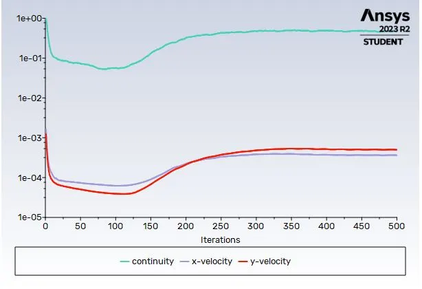
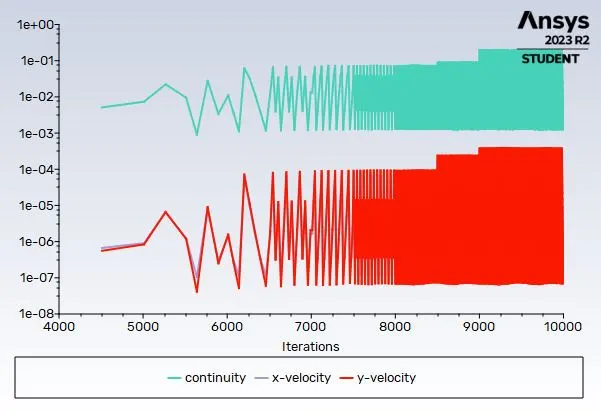
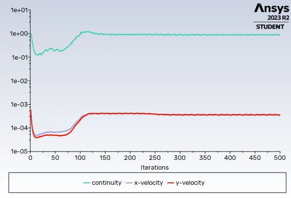
1. In both approaches, show that the flow has converged. That is, what quantities or plots need to be looked at to determine that the flow has converged?
2. Plots of the coefficient of drag and lift. 
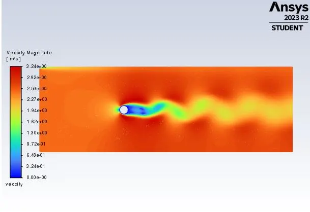
3. Plots to show vortex shedding behind the cylinder. 
4. Mention the referred material (Reference Paper or Fluid Mechanics Textbook) at the end of the challenge submission page. 

Answer:

Flow over a cylinder is a classic problem in fluid dynamics that helps us understand the behavior of fluids around objects with circular cross-sections. When a fluid (such as air or water) flows past a cylindrical object, several interesting phenomena occur, including the development of a flow pattern known as the Karman vortex street.

Here's a detailed explanation of the flow over a cylinder:

1. Stagnation Point and Separation Points:
• As the fluid approaches the cylinder, it encounters a point called the stagnation point where the flow velocity is reduced to zero. This is typically at the front face of the cylinder.
• As the fluid moves around the sides of the cylinder, it experiences a pressure gradient. Due to this pressure gradient, the fluid tends to follow the curvature of the cylinder. However, at some point, the fluid can no longer maintain this curved path and separates from the surface. These points are known as separation points.
2. Boundary Layer Formation:
• When the fluid flows over the surface of the cylinder, a boundary layer forms. This is a very thin layer of slow-moving fluid near the surface of the cylinder, which gradually accelerates until it reaches the free stream velocity further away from the surface.
3. Vortex Shedding:
• The most fascinating phenomenon in flow over a cylinder is the vortex shedding, which leads to the Karman vortex street.
• When the flow separates from the surface, it leaves behind a region of low pressure. This low-pressure region draws the surrounding fluid back towards the surface. Due to the curvature of the cylinder, the flow reattaches, creating a wake region behind the cylinder.
• As the flow continues past the cylinder, the boundary layer experiences oscillations, leading to the periodic shedding of vortices into the wake.
4. Karman Vortex Street:
• The shedding of these vortices alternates from one side of the cylinder to the other. This creates a pattern of alternating vortices that trail downstream.
• These vortices are called "Karman vortex street." They form in pairs, with one vortex spinning clockwise and the other counterclockwise.
• The shedding frequency (how often vortices are produced) is proportional to the flow velocity and the diameter of the cylinder.
5. Frequency of Vortex Shedding:
• The frequency at which vortices are shed is described by the Strouhal number (St), which is a dimensionless number. It is defined as the product of the frequency of vortex shedding, the cylinder diameter, and the fluid velocity. Mathematically, St = f * D / U, where f is the shedding frequency, D is the cylinder diameter, and U is the free stream velocity.
6. Application and Significance:
• Understanding flow over a cylinder and the phenomenon of Karman vortex street is crucial in various engineering applications, including designing structures like bridges, chimneys, and offshore platforms. It helps engineers predict and mitigate the effects of vortex-induced vibrations.

Procedure to solve the given problem in Ansys Fluent is described as follows:

1. Geometry

The schematcis of the flow domain id given as shown. 

 

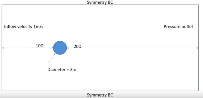
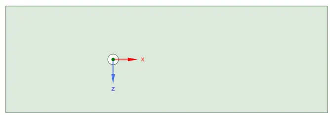
The geomerty is ctreated in the spaceclain as shown in the figure below with the flow domain dimension 20m*60m and the diameter of cylinder is taken as 2m.

2. Mesh

After the geometry is loaded we have to mesh it and here, the mesh size of  0.025m is used and the total number of elements are 40900.

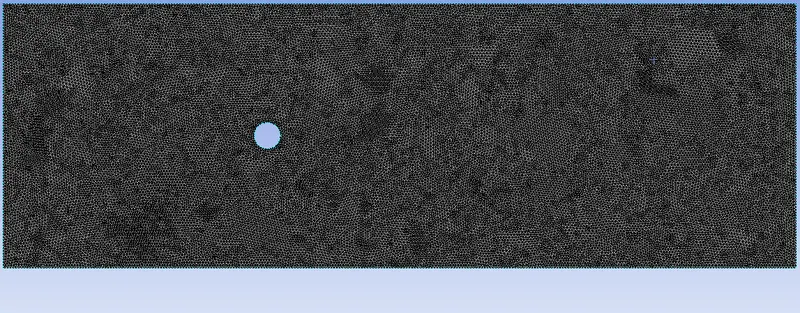
Here, the by default fluent has taken more number of quadrilateral cells than the triangular cells. So, we need to change it by clicking methods and choosing the triangluar cells in the insert option

The follwing steps are followed for meshing

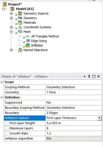
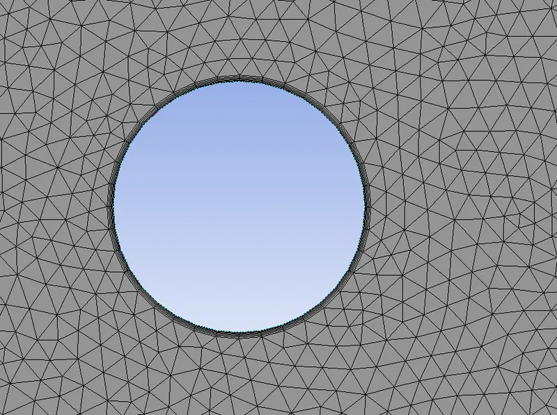
Then, inflation is added to create the body fitted mesh as shown: 

Here, 6 layers have been created. 

3. Setting up Ansys Fluent

 

 

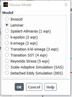
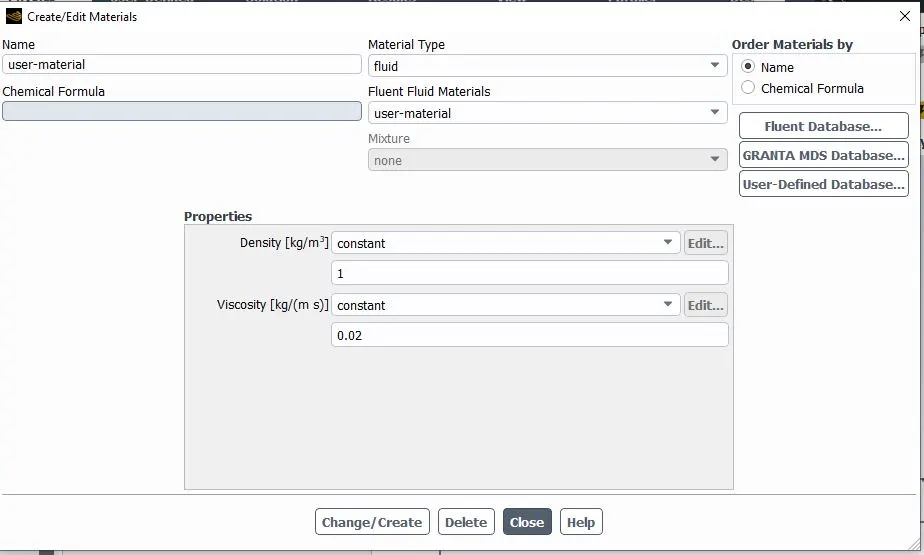
Part 1

Now, click on the boundary in the physics section and put the desired inlet velocity corresponding to the desired Renolds Number and perform the simulation for steady and unsteady  cases to complete the part one of the given problem.

Re = 100, density = 1 kg/m3, viscissity = 0.05 ps-s

This gives velocity as v = 2.5m/s

1. Steady Case

Residuals

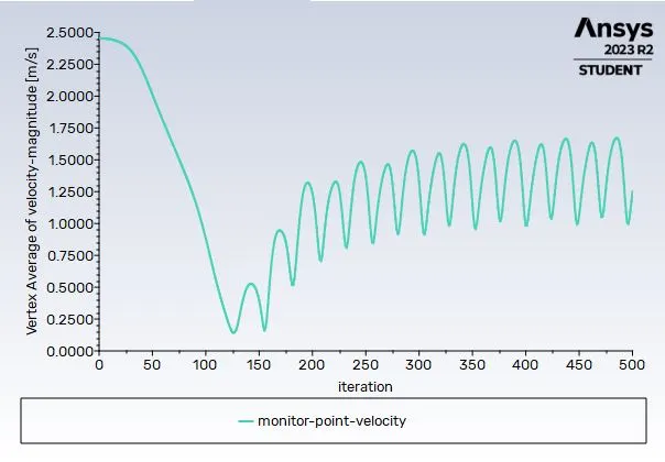
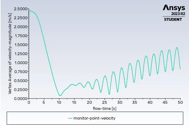
Monitor point velocity

 

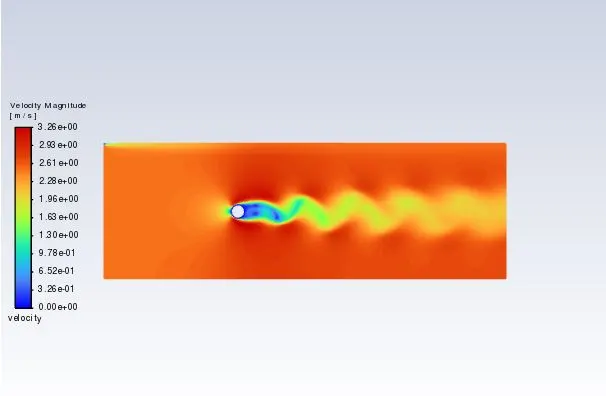
Velocity contour

 

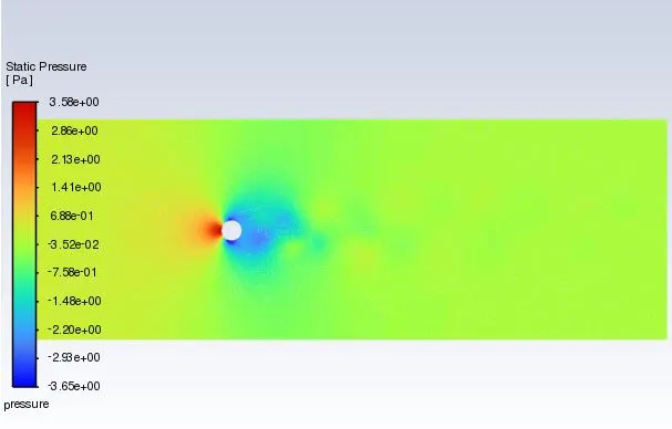
Pressure contour

 

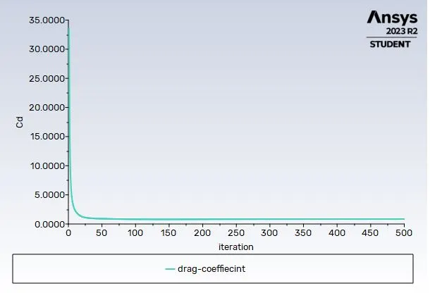
Drag Coefficient

 

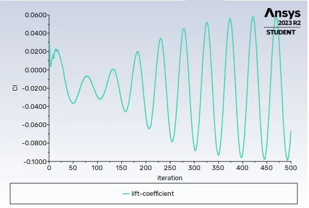
Lift Coefficient

 

2. Unstaedy Case

Residual

 

Monitor point velocity

 

Velocity contour

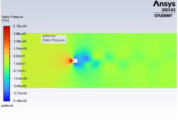
Pressure contour

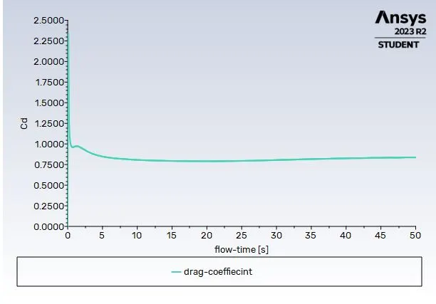
Drag Coefficient

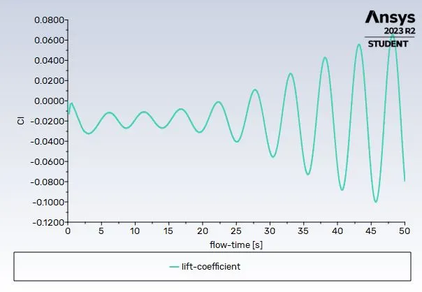
Lift Coefficient

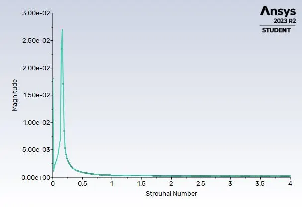
Strauhal number

 

Part 2

Steday state simulations

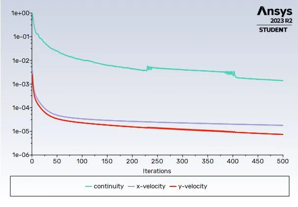
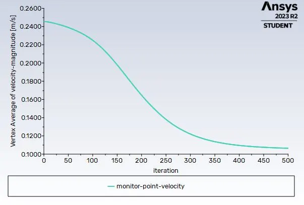
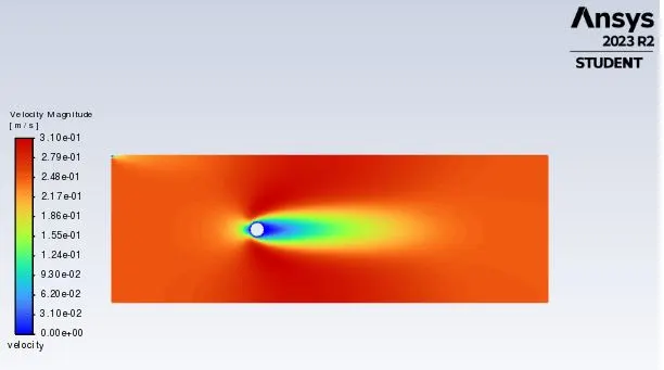
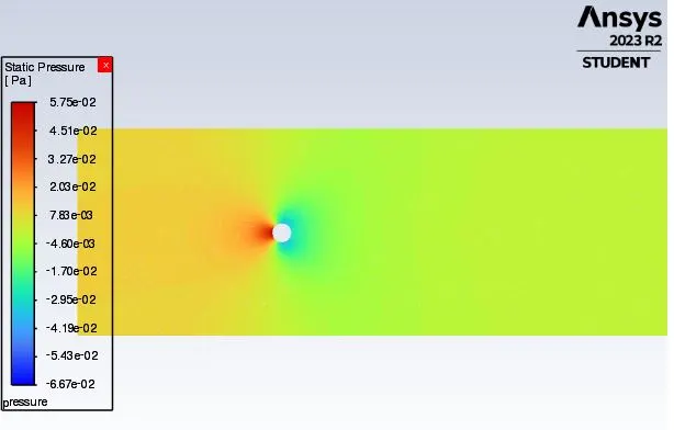
1. Re = 10, density = 1 kg/m3, viscissity = 0.05 ps-s

This gives velocity as v = 0.25m/s

Residulas

Monitor point velocity

Velocity contour

 

pressure contour

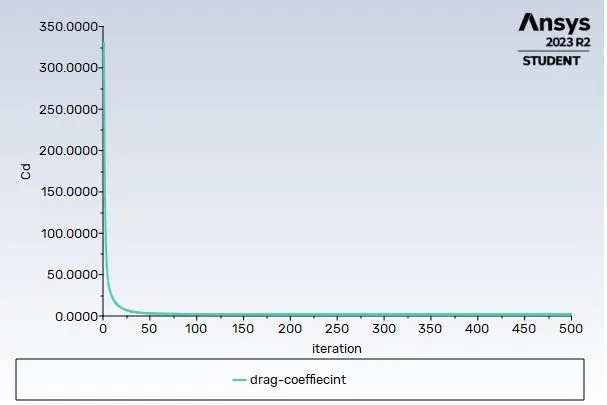
Drag coefficient

Lift coefficient

 

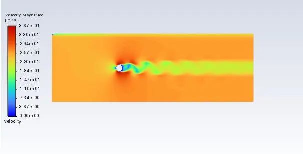
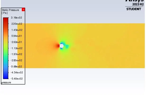
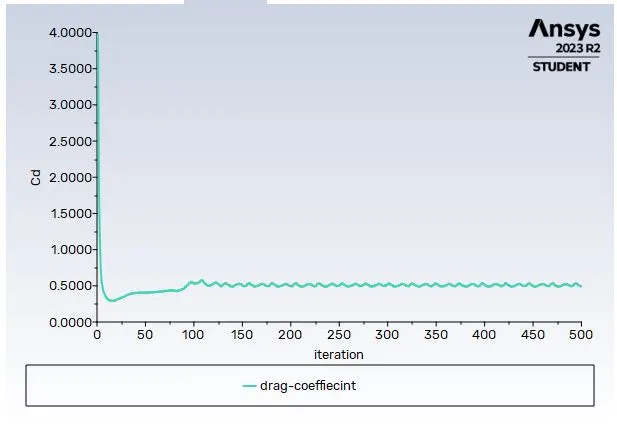
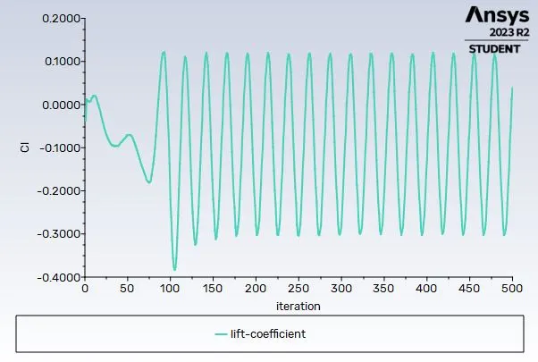
2. Re = 1000, density = 1 kg/m3, viscissity = 0.05 ps-s

This gives velocity as v = 25m/s

Residulas

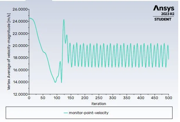
Monitor point velocity

Velocity contour

pressure contour

Drag coefficient

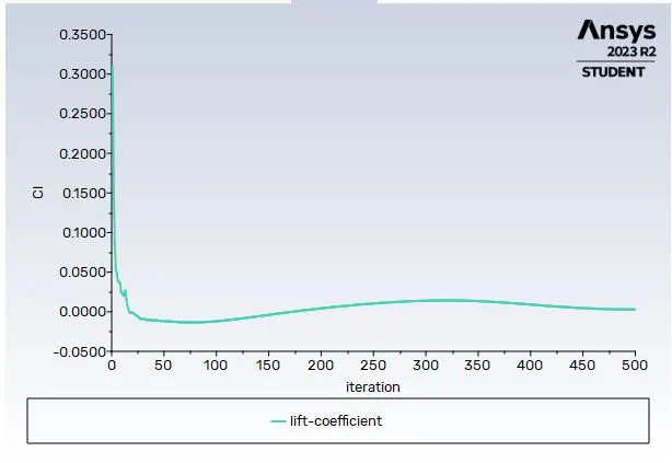
Lift coefficient

 

3. Re = 10000, density = 1 kg/m3, viscissity = 0.05 ps-s

This gives velocity as v = 250m/s

Residulas

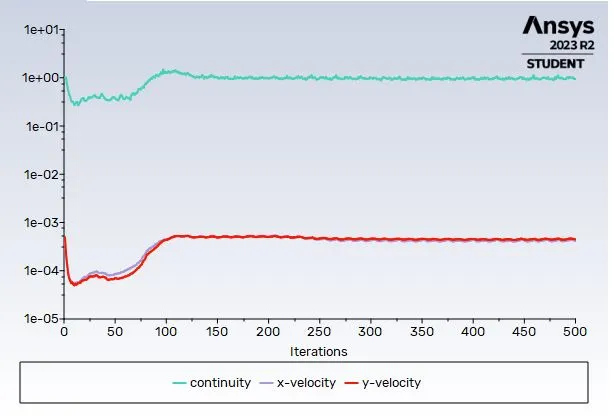
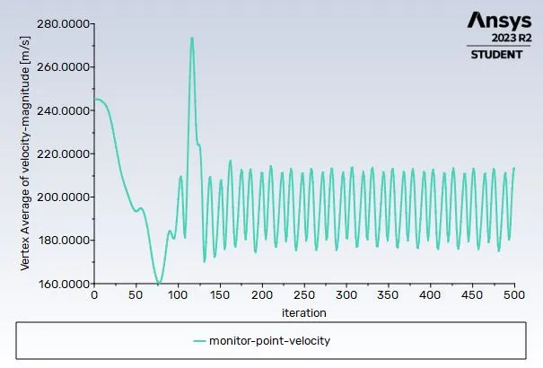
Monitor point velocity

Velocity contour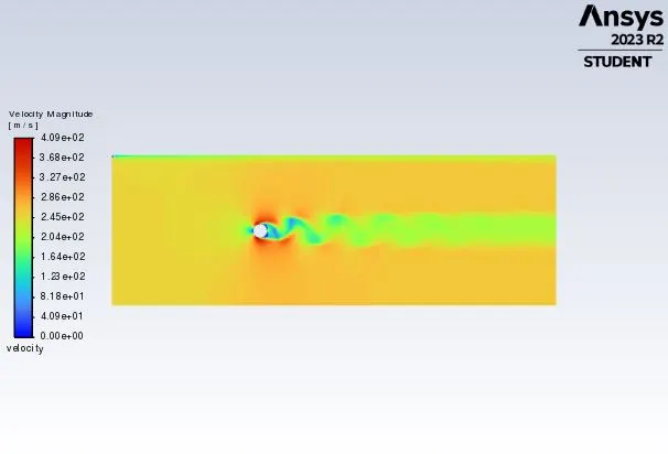

pressure contour

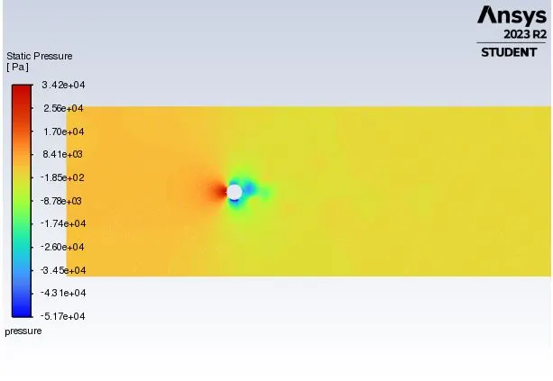
Drag coefficient

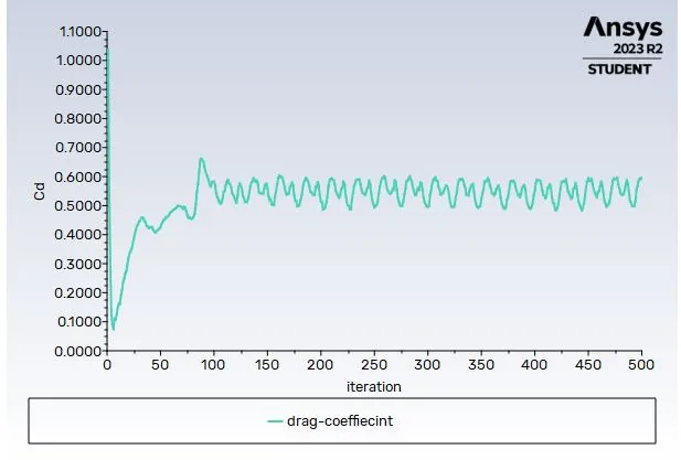
Lift coefficient

 

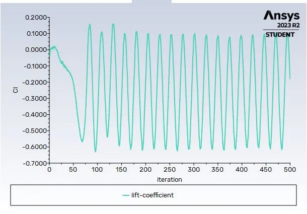
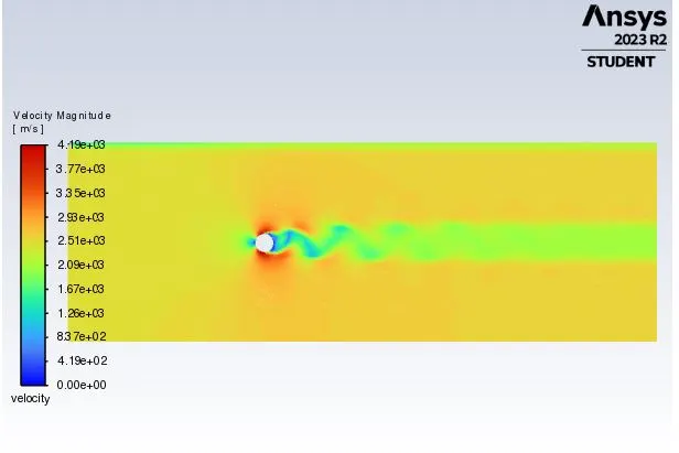
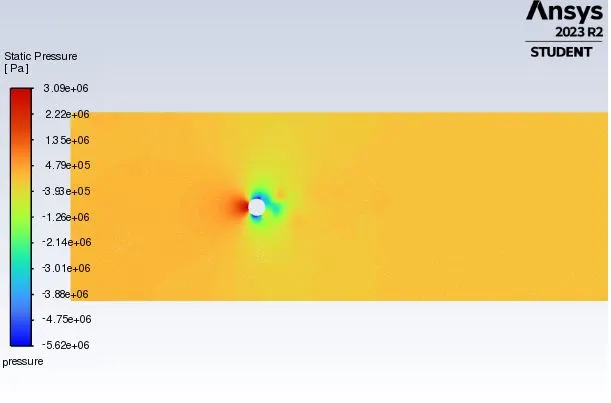
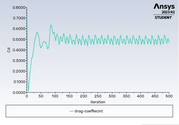
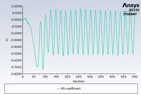
4. Re = 100000, density = 1 kg/m3, viscissity = 0.05 ps-s

This gives velocity as v = 2500m/s

Residual

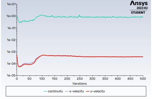
Monitor point veloccity

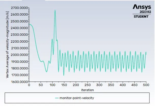
velocity contour

preesure contour

Drag coefficient 

Lift coefficient

 

Here is the Table which shows the brief summary of the all the cases simulated above:

RE	Cd	Cl
10 (Steady)	2.10	0.0029
100 (Steday	0.8583	-0.109
100 (Unsteady)	0.8365	-0.079
1000 (Staedy)	0.4944	0.038
10000 (Steady)	0.597	-0.078
100000 (Steady)	0.468	0.072

Reference

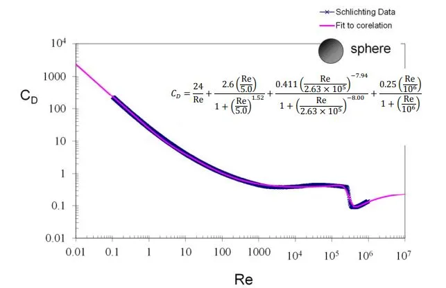
Morrison FA. Data correlation for drag coefficient for sphere. Department of Chemical Engineering, Michigan Technological University, Houghton, MI. 2013 Nov;49931.

Conclusion

1.When fluid flows over cylinder, wake region is formed next to cylinder due to decrease in pressure and recirculation of flow occures and hence flow separation occures.

2.We are unable to observe flow separation at low reynolds no., for example Re at around 50, as flow over cylinder is transient meaning time dependent phenomenon. 

3. In this assignment, all parameters were held constant; only the velocity was changed to alter Reynolds number. Therefore, the coefficient of drag reduces as the Reynolds number rises. At around Reynolds number = 4000 there is transition from laminar to turblent flow is seen due to  which there is slight increase in coefficient of drag is seen.

4. Strauhal number is 0.125 for an unsteady condition with Reynolds number equal to 100.