Rayleigh Taylor Instability

Aim: To perform Rayleigh-Taylor instability CFD simulations.

Objectives:

1. To develop a numerical case set-up for Rayleigh-Taylor instability problem in Ansys Fluent.

2. To understand the effect of variation in Atwood number on RT instabilities.

Introduction:

The Rayleigh-Taylor instability is a fundamental fluid dynamics phenomenon that occurs when there is an interface between two fluids of different densities, and the denser fluid is placed above the lighter fluid. This instability leads to the mixing of the two fluids and is observed in a wide range of natural and engineered systems.
From a computational fluid dynamics (CFD) point of view, simulating the Rayleigh-Taylor instability involves solving the Navier-Stokes equations coupled with the continuity equation. These equations describe the conservation of momentum and mass in a fluid, respectively.

Rayleigh-Taylor instability from a CFD perspective:

1. Initial Conditions:
• You start by defining the initial conditions of the problem. This includes specifying the densities, velocities, and pressures of the two fluids, as well as the geometry and boundary conditions of the system.
2. Grid Generation:
• The computational domain is discretized into a grid or mesh. The choice of grid type and resolution is crucial for accurately capturing the details of the instability. The grid should be fine enough to resolve the interface and capture the turbulent structures that develop.
3. Governing Equations:
• The Navier-Stokes equations and continuity equation are solved numerically within the computational domain. These equations describe the conservation of mass, momentum, and energy in the fluid.
4. Boundary Conditions:
• Proper boundary conditions need to be applied to mimic the physical constraints of the problem. This includes specifying the velocities, pressures, or other relevant quantities at the boundaries.
5. Density and Pressure Formulation:
• The Rayleigh-Taylor instability is often characterized by differences in density and pressure across the interface. In CFD simulations, an equation of state is used to relate density and pressure based on the properties of the fluids.
6. Time Integration:
• The simulation progresses in time steps. Different time integration schemes, such as explicit or implicit methods, can be used to update the solution from one time step to the next.
7. Turbulence Modeling:
• If the flow becomes turbulent, additional models for turbulence (like the Reynolds-averaged Navier-Stokes or Large Eddy Simulation models) may be employed to account for the effects of small-scale turbulence on the large-scale flow structures.
8. Visualization and Analysis:
• Post-processing involves visualizing and analyzing the simulation results. This can include generating plots, images, and videos to understand the evolution of the instability

Some practical CFD models that have been based on the mathematical analysis of Rayleigh Taylor Instability

1. Kelvin-Helmholtz/Rayleigh-Taylor (KH-RT) Model:

• This model combines the effects of the Kelvin-Helmholtz instability (for sheared flows) and the Rayleigh-Taylor instability (for density differences). It's particularly relevant for situations where there is both velocity shear and a density gradient, such as in astrophysical and laboratory plasmas.

2. Lattice Boltzmann Method (LBM):

• LBM is a numerical method used in CFD. It has been adapted to study multiphase flows, including those with Rayleigh-Taylor instability. By discretizing the Boltzmann transport equation, LBM can capture complex fluid behaviors, including instabilities.

3. Volume-of-Fluid (VOF) Method:

• The VOF method tracks the interface between different fluids by solving a fraction field, representing the volume fraction of each fluid. This approach has been extended to study Rayleigh-Taylor instabilities, allowing for the prediction of interface dynamics and mixing.

4. Reynolds-Averaged Navier-Stokes (RANS) Models:

• Turbulence models within the RANS framework, like the k-ε and k-ω models, have been applied to study turbulent flows involving Rayleigh-Taylor instabilities. These models provide closure for the turbulence equations and are valuable for simulating high Reynolds number flows.

5. Large Eddy Simulation (LES):

• LES resolves large-scale turbulent structures while modeling the smaller ones. It has been employed to capture the turbulence generated by Rayleigh-Taylor instabilities, providing a detailed representation of the flow field.

In the present study, two cases are performed for Rayleigh-Taylor instability problem in which density of the lighter fluid is varried and the results and animations are recorded.

Case 1: Water and Air

Geometry: Two patches of different fluids (water and air) of appropriate dimmensions (20 mm*20 mm) are sketched.

Meshing: Mesh size of 0.25 mm is taken and mesh is generated.

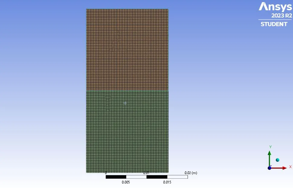
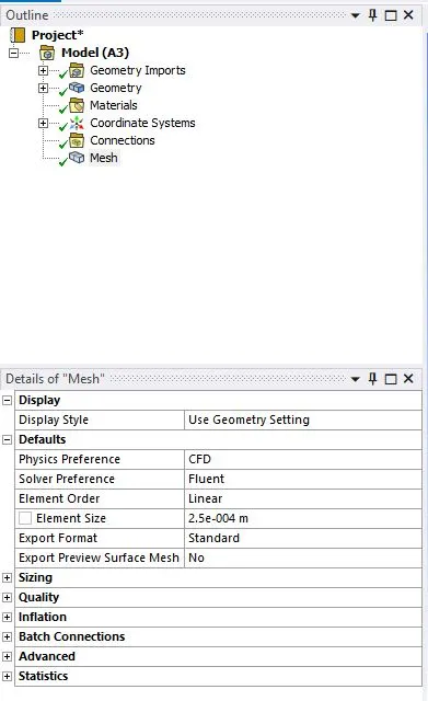
After meshing is done, physics is set up in the Ansys Fluent.

Laminal Viscous model is used as the process of mixing is very slow.

Transient Simiulation is performed

Materials are then selected (water and air in this case)

Standard Initilization is done.

The most important thing which needs to be taken care of just after Standard Initilization is the Patching work.

Patch is done betwen the two fluids and the calculation part follows.

The simulation is run with time step = 0.001s and the observation is recorded.

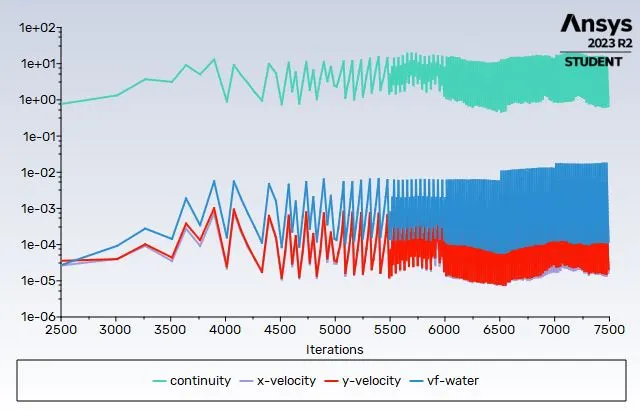
Residuals:

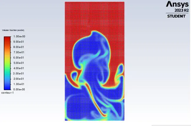
Snips from the intermediate simulation:

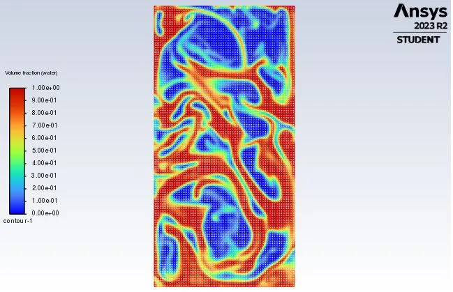
Link for the animation for case 1:

https://drive.google.com/file/d/1IzQQKT6DYRVPQsmcEouB67YF-JRwuFGf/view?usp=sharing

Case 2: Water and user defined material

Density of the user defined materials = 400 kg/m³

Viscosity = 0.001 kg/m-s

All the processes from geometry creation to setting up the physics in the Ansys Fluent will remain same as in previous case except for the material selection for the lighter fluid which has to be defined by the user (user defined material with given properties in the problem).

The simulation is run with the same time step = 0.001s and the observation is recorded.

Residuals:

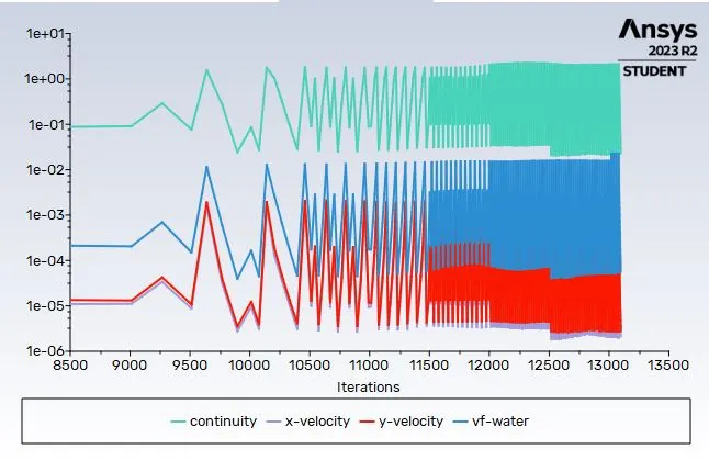
Snips from the intermediate simulation:

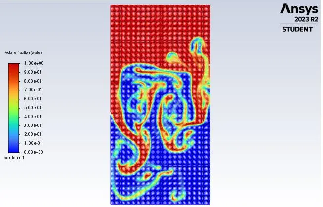
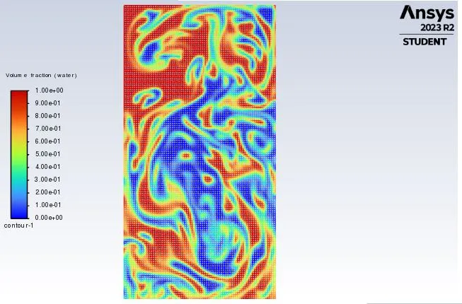
Link for the animation for case 2:

https://drive.google.com/file/d/1avo8Du4zvszOZY7McT0kMsA9GL-SSliE/view?usp=sharing

Atwood Number:

The Atwood number (A) is a dimensionless number in fluid dynamics used in the study of hydrodynamic instabilities in density stratified flows. It is a dimensionless density ratio defined as:

A = (ρ₁ - ρ₂)/ (ρ₁+ ρ₁)

For the above cases:

Case 1:

Heavier fluid (water), ρ₁ = 998.2 kg/m³

Lighter fluid (air), ρ₂ = 1.225 kg/m³

Therefore, Atwood number, A = 0.996

Case 2:

Heavier fluid (water), ρ₁ = 998.2 kg/m³

Lighter fluid (user-defined material), ρ₂ = 400 kg/m³

Therefore, Atwood number, A = 0.427

Observations:

• The evolution of interface grows faster with increase in Atwood number.
• Larger Atwood number results in larger amplitude of perturbation.

• When Atwood number close to 1, the much lighter fluid below the heavier fluid takes the form of larger bubble-like plumes.