Simulation of a 1D Super-sonic nozzle flow simulation using Macormack Method
Problem Definition
We have to simulate the isentropic flow through a quasi 1D subsonic-supersonic nozzle.
We will derive both the conservation and non-conservation forms of the governing equations and solve them using MacCormack's technique.
We need to determine the steady-state temperature distribution for the flow-field variables and investigate the difference between the two forms of governing equations by comparing their solutions.
Introduction
A subsonic-supersonic flow nozzle is a type of nozzle in which the inlet throat has Mach number below 1, at the throat, it is equal to 1 and in the divergent outlet region, it is greater than 1.
Assumption
We consider the steady, isentropic flow through a convergent-divergent nozzle. The flow at the inlet to the nozzle comes from a reservoir where the pressure and temperature are `P_o`and `T_o` respectively. The cross-sectional area of the reservoir is large and hence the velocity is very small. Thus `P_o`and `T_o` are the stagnation values or total pressure and total temperature respectively.
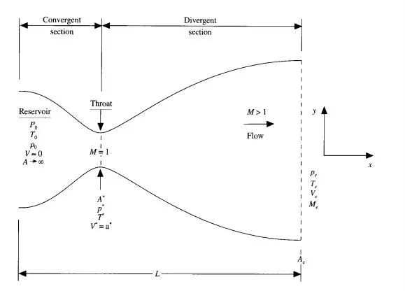
The flow expands isentropically to supersonic speed at the nozzle exit. The flow is locally subsonic in the convergent section of the nozzle, sonic at the throat, and supersonic at the divergent section. The sonic flow at the throat means that the local velocity at this location is equal to the local speed of the sound.
We are assuming that the properties vary only with the x-axis, such flow is defined as quasi-one-dimensional flow.
Governing Equations
Non-dimensional quantities
We are using the non dimensional quantities to solve the problem.
Temperature `T^' = T/T_o`
Density `rho^' = rho/rho_o`
Distance `x^' = x/L`
Area A' = A/A*
velocity `v^' = v/a_o` where `a_o`is the local sonic velocity
time `t^' = t/(L/a_o)` where `L/a_o` is the characterstic time scale
Non-conservative form
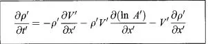
(i) continuty equation
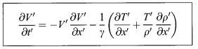
(ii) Momentum equation
(iii) Energy equation

Conservative form
(i) continuty equation
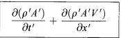 =0
=0
(ii) Momentum equation

(iii) Energy equation

MacCormack's Method
To calculate the numerical solution we are going to use MacCormack's technique. The MacCormack method is a variation of the two-step lax-Wendorff scheme but is much simpler in the application.
The application of the MacCormack method to the above equation proceeds in two steps; a predictor step which is followed by a corrector step.
Predictor step: In the predictor step, a "provisional" value of u at time level n+1 (denoted by  ) is estimated to obtained by replacing the spatial and temporal derivatives in the previous first-order hyperbolic equation using a forward differencing scheme.
Corrector step: In the corrector step, the predicted value is corrected according to the equation. In the corrector step, we use a backward differencing scheme.
After that, we calculate the average value and solve the equation.
Discretization Procedure
Non-conservative form
(i) continuity equation
Applying forward differencing for predictor calculation

where:-
`rho_i^t`= density at node i at time step t
`rho_(i+1)^t`= density at node i+1 at time step t
`v_(i+1)^t`= velocity at node i+1 at time step t
`v_i^t` = velocity at node i at time step t
`A_(i+1)^t` = area at node i+1 at time step t
`A_i^t`= area at node i at time step t
`trianglex`= x-axis grid space
Applying backward differencing for corrector calculation
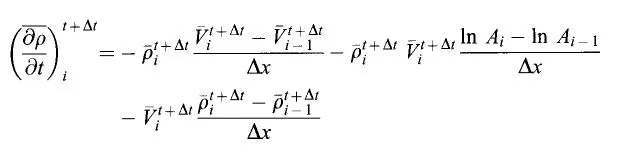
where:-
`rho_i^(t+trianglet)`= density at node i at time step `(t+trianglet)`
`rho_(i-1)^(t+trianglet)`= density at node i-1 at time step `(t+trianglet)`
`v_(i-1)^(t+trianglet)`= velocity at node i-1 at time step `(t+trianglet)`
`v_i^(t+trianglet)` = velocity at node i at time step`(t+trianglet)`
`A_(i-1)^(t+trianglet)` = area at node i-1 at time step `(t+trianglet)`
`A_i^(t+trianglet)`= area at node i at time step `(t+trianglet)`
`trianglex`= x-axis grid space
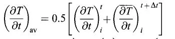
Average of both values
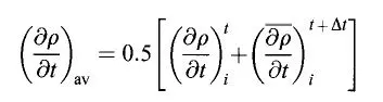
(ii) Momentum equation
Applying forward differencing for predictor calculation

where:-
`rho_i^t`= density at node i at time step t
`rho_(i+1)^t`= density at node i+1 at time step t
`v_(i+1)^t`= velocity at node i+1 at time step t
`v_i^t` = velocity at node i at time step t
`A_(i+1)^t` = area at node i+1 at time step t
`A_i^t`= area at node i at time step t
`T_i^t`= temperature at node i at time step t
`T_(i+1)^t`= temperature at node i+1 at time step t
`trianglex`= x-axis grid space
`gamma`= gamma
Applying backward differencing for corrector calculation

where:-
`rho_i^(t+trianglet)`= density at node i at time step `(t+trianglet)`
`rho_(i-1)^(t+trianglet)`= density at node i-1 at time step `(t+trianglet)`
`v_(i-1)^(t+trianglet)`= velocity at node i-1 at time step `(t+trianglet)`
`v_i^(t+trianglet)` = velocity at node i at time step`(t+trianglet)`
`T_(i-1)^(t+trianglet)` = temperature at node i-1 at time step `(t+trianglet)`
`T_i^(t+trianglet)`= temperature at node i at time step `(t+trianglet)`
`trianglex`= x-axis grid space
`gamma`= gamma
Average of both values
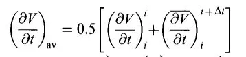
(iii) Energy equation
Applying forward differencing for predictor calculation

where:-
`v_(i+1)^t`= velocity at node i+1 at time step t
`v_i^t` = velocity at node i at time step t
`A_(i+1)^t` = area at node i+1 at time step t
`A_i^t`= area at node i at time step t
`T_i^t`= temperature at node i at time step t
`T_(i+1)^t`= temperature at node i+1 at time step t
`trianglex`= x-axis grid space
`gamma`= gamma
Applying backward differencing for corrector calculation
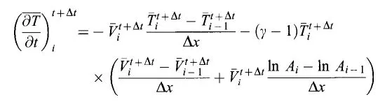
where:-
`rho_i^(t+trianglet)`= density at node i at time step `(t+trianglet)`
`rho_(i-1)^(t+trianglet)`= density at node i-1 at time step `(t+trianglet)`
`v_(i-1)^(t+trianglet)`= velocity at node i-1 at time step `(t+trianglet)`
`v_i^(t+trianglet)` = velocity at node i at time step`(t+trianglet)`
`T_(i-1)^(t+trianglet)` = temperature at node i-1 at time step `(t+trianglet)`
`T_i^(t+trianglet)`= temperature at node i at time step `(t+trianglet)`
`A_(i-1)^(t+trianglet)` = area at node i-1 at time step `(t+trianglet)`
`A_i^(t+trianglet)`= area at node i at time step `(t+trianglet)`
`trianglex`= x-axis grid space
`gamma`= gamma
Average of both values
Conservative form
To solve the conservative form of the nozzle equation we are going to convert it into the generic form of the governing equation.
So we are going to define the elements of the solution vector U, the flux vector F, and source term J as follows:-
Solution vector:-
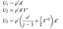
where:-
`rho^'`=density
`A^'`= area
`V^'`velocity
`e^'`=energy
`gamma`=gamma
flux vector:-
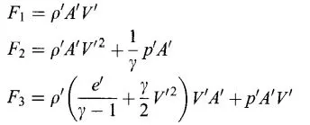
where:-
`rho^'`=density
`A^'`= area
`V^'`velocity
`e^'`=energy
`gamma`=gamma
`p^'`= pressure
Source term:-
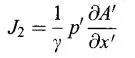
where:-
`p^'`= pressure
`partialA^'`= area difference
`partialx^'`= x-axis grid differencing
`gamma`=gamma
Now Governing equation can be written like this:-
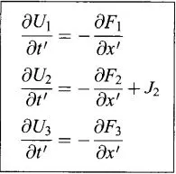
Now with the help of these equations, we are going to solve the governing equation that I will explain in the Matlab script explanation.
Initial and Boundary Conditions
In the numerical solution boundary and initial conditions are the important aspects. Because without the physical implementation of boundary conditions we can't calculate the proper numerical solution to our flow problem.
For Non-conservative form
(i) Boundary Condition
In the current problem, the grid point 1 and N is the two boundary points on the x-axis. Point 1 is the inflow boundary, with the flow coming from the reservoir and entering in the nozzle and point N is the outflow boundary, with flow leaving the nozzle at the nozzle exit.
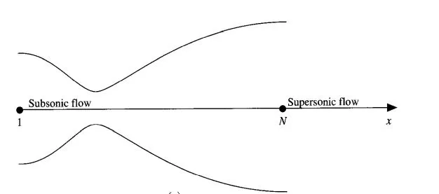
At point 1 the flow is subsonic so that's why this is the subsonic inflow boundary and at point N the flow is supersonic so that's why this is the supersonic outflow boundary.
The unsteady and inviscid flow is governed by hyperbolic equations and therefore for one-dimensional unsteady flow there exist only two real characteristic lines in xt plane.
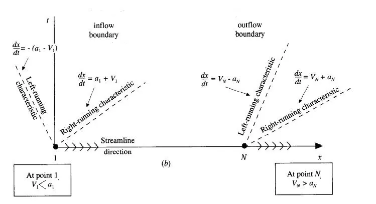
At point 1 the local flow velocity is subsonic, `v_1 that's why the left running characteristic at point 1 propagating out of the domain and the right-running characteristic is propagating to the right into the domain. So this tells us that when one characteristic propagates into the domain then the value of one dependent flow-field variable must be allowed to float at the boundary. So we are going to held `rho^' and T^'` and allow`V^'`to float.
So at point 1
`rho_1`= 1
`T_1` = 1
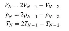
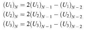
At point N both left and right running characteristic are going out of the domain so all variables must be allowed to float at this boundary
at point N
(ii) Initial Condition
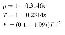
To start the time marching calculation we must stipulate initial conditions for `rho, T, and V` at time t=0.
We are going to need the following initial conditions:-
For Conservative form
(i) Boundary Condition
The boundary conditions for the conservative form theoretically the same as the non-conservative form. We are going to held `rho^' and T^'` and allow`V^'`to float.
Because `rho^' and T^'` are fixed U1 will be fixed
`U_1 = rho^'*A^'`= fixed
And because `V^'` is floating the value of `U_2 and U_3`will be floating.
`(U_2)_(i=1)=2*(U_2)_(i=2)-(U_2)_(i=3)`
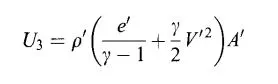
At point N the boundary condition will be this:-
(ii) Initial Condition
We need the initial values of `U_1,U_2 and U_3` at time t=0. So we are going to need the `rho^' and T^'` value to calculate `U_1,U_2 and U_3`.
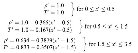
and the velocity will be calculated by this formula:-
`V^' = 0.59/(rho^'*A^')`
Now we can calculate the`U_1,U_2 and U_3` at time t=0.
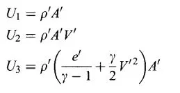
where `e^' = T^'`
Time step calculation
In this case we are going to calculate the time step by the following steps:-
First we are going to calculate dt at every grid points
`dt=C*((trianglex)/(a+v))`
where:- C = courant number
`triangle x`= grid spacing
a = sound speed
v = velocity
So we have taken the courant number 0.5. And now with this courant number, we have calculated the time step at every grid point.
Now we are going to take the minimum value of dt from all the grid point dt value.

Matlab Script
For the solution quasi 1D subsonic-supersonic nozzle. We are going to solve the conservative and non-conservative form of the governing equation. For that, I have created the following code
clear all
close all
clc


%input
n = 31;
x = linspace(0,3,n);
dx = x(2)-x(1);

%throat
throat = (n-1)/2+1;
%gamma
gamma = 1.4;
% Courant number
C = 0.5;
% number of Time loop
nt = 1400;
l = 1:nt;

% non conservation solution
m1 = non_conservation_solution(n,x,dx,throat,gamma,C,nt,l);

% conservation solution
m2 = conservation_solution(n,x,dx,throat,gamma,C,nt,l);


figure(9)
plot(x,m1)
hold on
plot(x,m2)
legend('non conservation form','conservation form')
title('mass flow rate comparison')
xlabel('x axis')
ylabel('mass flow rate')
Matlab Script explanation:-
1. First we are going to need some input to solve the problem.
Number of grid points n= 31
Domain x = linspace(0,3,n)
Grid space dx = x(2)-x(1)
We are going to calculate the throat where the area will be 1. Which is at the mid point of the grid. So
'throat =`(n-1)/2+1`'
gamma = 1.4
Courant number C = 0.5
Number of Time loop nt = 1400
2. Now we are going to calculate the mass flow rate, density, temperature, pressure, and Mach number for non-conservative form. So that we can compare that to the mass flow rate of the conservative form. To do that we are going to call a function 'non_conservation_solution'
[m1,rho1,T1,P1,M1] = non_conservation_solution(n,x,dx,throat,gamma,C,nt,l);
Function:-
function [m,rho,T,P,M] = non_conservation_solution(n,x,dx,throat,gamma,C,nt,l)

% calculating initial profile
rho = 1-0.3146*x;
T = 1-0.2314*x;
v = (0.1+1.09*x).*T.^0.5;


%area
a = 1+2.2*(x-1.5).^2;
% sound velocity
s = T.^0.5;

    %time step
    for p = 1:n
        dt(p) = C*(dx/(s(p)+v(p)));
        dt_p(p) = dt(p);
        dt = min(dt_p);
    end

%outer time loop
for k = 1:nt

    rho_old = rho;
    v_old = v;
    T_old = T;

    %predicted method
   for j = 2:n-1
       dvdx = (v(j+1)-v(j))/dx;
       drhodx = (rho(j+1)-rho(j))/dx;
       dTdx = (T(j+1)-T(j))/dx;
       dlogadx = (log(a(j+1))-log(a(j)))/dx;

       %continuity equation
       drhodt_p(j) = -rho(j)*dvdx -rho(j)*v(j)*dlogadx -v(j)*drhodx;

       % Momentum equation
       dvdt_p(j) = -v(j)*dvdx -(1/gamma)*(dTdx +(T(j)/rho(j))*drhodx);

       % Energy equation
       dTdt_p(j) = -v(j)*dTdx -(gamma-1)*T(j)*(dvdx +v(j)*dlogadx);

       %solution update
       rho(j) = rho(j) + drhodt_p(j)*dt;
       v(j) = v(j) + dvdt_p(j)*dt;
       T(j) = T(j) + dTdt_p(j)*dt;
   end

     %corrector method
      for j = 2:n-1
           dvdx = (v(j)-v(j-1))/dx;
           drhodx = (rho(j)-rho(j-1))/dx;
           dTdx = (T(j)-T(j-1))/dx;
           dlogadx = (log(a(j))-log(a(j-1)))/dx;

           %continuity equation
           drhodt_c(j) = -rho(j)*dvdx -rho(j)*v(j)*dlogadx -v(j)*drhodx;

           % Momentum equation
           dvdt_c(j) = -v(j)*dvdx -(1/gamma)*(dTdx +(T(j)/rho(j))*drhodx);

           % Energy equation
           dTdt_c(j) = -v(j)*dTdx -(gamma-1)*T(j)*(dvdx +v(j)*dlogadx);

      end

      % Compare the average time derivative

      drhodt = 0.5*(drhodt_p +drhodt_c);
      dvdt = 0.5*(dvdt_p + dvdt_c);
      dTdt = 0.5*(dTdt_p + dTdt_c);

      % final solution update
      for i = 2:n-1
          rho(i) = rho_old(i) + drhodt(i)*dt;
          v(i) = v_old(i) + dvdt(i)*dt;
          T(i) = T_old(i) + dTdt(i)*dt;

      end

      % Apply the boundary condition
      % inlet
      v(1) = 2*v(2) - v(3);

      % outlet
      v(n) = 2*v(n-1) - v(n-2);
      rho(n) = 2*rho(n-1) - rho(n-2);
      T(n) = 2*T(n-1) - T(n-2);

      %Mach number
      M = v./(T.^0.5);
      %mass flow rate
      m = rho.*a.*v;
      %pressure ratio
      P = rho.*T;

     % when area is 1
     M_at1(k) = M(throat);
     rho_at1(k) = rho(throat);
     T_at1(k) = T(throat);
     P_at1(k) = P(throat);
     %for residual plot
     drhodt_at1(k) = abs(drhodt(throat));
     dvdt_at1(k) = abs(dvdt(throat));
     dTdt_at1(k) = abs(dTdt(throat));

     %mass flow rate at various time step
    if k==50
        figure(1)
        plot(x,m,'linewidth',3)
        hold on
        elseif k==100
          plot(x,m,'linewidth',3)
        elseif k==150
          plot(x,m,'linewidth',3)
        elseif k==200
          plot(x,m,'linewidth',3)
        elseif k==700
         plot(x,m,'linewidth',3)
         xlabel('x axis')
         ylabel('mass flow rate')
         legend('at 50 time step','at 100 time step','at 150 time step','at 200 time step','at 700 time step')
         title_text = sprintf('Variation of Mass flow rate distribution at different time steps n non conservation form');
         title(title_text)
    end

end


      %plotting
      figure(2)
      subplot(4,1,1)
      plot(x,M)
      xlabel('x axis')
      ylabel('Mach number')
      title('steady state values of non conservation form')

      subplot(4,1,2)
      plot(x,P)
      xlabel('x axis')
      ylabel('pressure')

      subplot(4,1,3)
      plot(x,rho)
      xlabel('x axis')
      ylabel('density')


      subplot(4,1,4)
      plot(x,T)
      xlabel('x axis')
      ylabel('Temperature')

      figure(3)
      subplot(4,1,1)
      plot(l,rho_at1)
      xlabel('Time step')
      ylabel('density')
      title('time wise variation of variables in non conservation form')

      subplot(4,1,2)
      plot(l,T_at1)
      xlabel('Time step')
      ylabel('temperature')


      subplot(4,1,3)
      plot(l,P_at1)
      xlabel('Time step')
      ylabel('pressure')

      subplot(4,1,4)
      plot(l,M_at1)
      xlabel('Time step')
      ylabel('Mach number')

      figure(4)
      semilogy(l,drhodt_at1,'r')
      hold on
      semilogy(l,dTdt_at1,'g')
      semilogy(l,dvdt_at1,'k')
      xlabel('Time step')
      ylabel('Residual')
      title('non conservation form')
      legend('drhodt','dTdt','dvdt')

end
Function explanation:-
- First, we are going to calculate `rho`,T and v at the time t=0. For that, we are going to use a formula that I have explained in the initail condition of the non-conservative form.
- Now we are going to calculate the area `a = 1+2.2*(x-1.5)^2`
- Now we are calculating sound velocity`s = T^0.5`
- Now we are going to calculate the time step dt which I have explained above.
- Now we are going to need a time loop. 'for k = 1:nt'
- We are going to make a copy of the `rho`,T and v array. Because we are going to need it in the updated solution.
- Now we are going to calculate the predicted values. For that, we are going to use'for loop'.
- In the calculation of the predicted value, we are going to use forward differencing. Which I have explained in the discretization.
- Now we are going to update our `rho`,T and v values.
- Now we are going to calculate the corrector values. For that, we are going to use 'for loop'.
- In the calculation of the corrected value, we are going to use backward differencing. Which I have explained in the discretization.
- Now we are going to calculate the average value of the predicted and corrector values.
- Now we are going to update the final solution. Which we are going to calculate the all inner points of the grid.
- `rho = rho_(old)+ (drho)/dt*dt`
- `v = v_(old) + (dv)/dt*dt;`
- `T = T_(old) + (dT)/dt*dt;`
- Now we are going to apply the inner and outer boundary conditions.
- Now we are going to calculate the Mach number. `M = v/T^0.5`
- Now we are going to calculate the mass flow rate. `m = rho*a*v`
- Now we are going to calculate pressure. `P = rho*T`
- We want to plot the graph of the Mach number, density, temperature, and pressure values of the throat at different time steps. So we are going to store them.
- For residual graph we are going to need `((partialrho)/(partialt))_(avg)`, `((partialv)/(partialt))_(avg)` and `((partialT)/(partialt))_(avg)`values of throat at every time step.
- Now we are going to plot the mass flow rate at a different time step. I have plotted the graph at time step 50, 100, 150, 200, and 700. Now we end our time loop
- Now we are going to use subplot to plot the final values of Mach number, pressure, density, and temperature with the x-axis.
- Now we are going to use subplot to plot the throat values of Mach number, pressure, density, and temperature at a different time step.
- Now we are going to plot the residual plot, for which we are going to use the semiology command. We are going to plot `((partialrho)/(partialt))_(avg)`, `((partialv)/(partialt))_(avg)` and `((partialT)/(partialt))_(avg)`.
- Now we are going to end the function.
3. Now we are going to calculate the mass flow rate, density, temperature, pressure, and Mach number for conservative form. To do that we are going to call a function 'conservation_solution'.
'[m2,rho2,T2,P2,M2] = conservation_solution(n,x,dx,throat,gamma,C,nt,l);'
function [m,rho,T,P,M] = conservation_solution(n,x,dx,throat,gamma,C,nt,l)

% calculating initial profile
for i = 1:n
    if (x(i)>=0 && x(i)<=0.5)
        rho(i) = 1;
        T(i) = 1;
    end

    if (x(i)>=0.5 && x(i)<=1.5)
        rho(i) = 1-0.366.*(x(i)-0.5);
        T(i) = 1-0.167.*(x(i)-0.5);
    end

    if (x(i)>=1.5 && x(i)<=3)
        rho(i) = 0.634-0.3879.*(x(i)-1.5);
        T(i) = 0.833-0.3507.*(x(i)-1.5);
    end
end

%area
a = 1+2.2*(x-1.5).^2;
%velocity
v = .59./(rho.*a);
% sound velocity
s = T.^0.5;

%solution vector
U1 = rho.*a;
U2 = 0.59*ones(1,n);
U3 = rho.*a.*((T./(gamma-1))+((gamma/2).*(v.^2)));


    %time step
    for p = 1:n
        dt(p) = C*(dx/(s(p)+v(p)));
        dt_p(p) = dt(p);
        dt = min(dt_p);
    end

% %outer time loop
for k = 1:nt

        U1_old = U1;
        U2_old = U2;
        U3_old = U3;

        % flux vector
        F1 = U2;
        term1 = (U2.^2)./U1;
        term2 = (gamma-1)/gamma;
        F2 = term1+term2.*(U3-(gamma/2).*term1);
        term3 = (gamma.*U2.*U3)./U1;
        term4 = (gamma*(gamma-1))/2;
        term5 = (U2.^3)./(U1.^2);
        F3 = term3-term4.*term5;

        % source term
        for o = 1:n-1
            J2(o) = (1/gamma)*rho(o)*T(o)*((a(o+1)-a(o))/dx);
        end

        %predicted method
    for j = 2:n-1

        dU1dt_p(j) = -(F1(j+1)-F1(j))/dx;
        dU2dt_p(j) = -(F2(j+1)-F2(j))/dx+J2(j);
        dU3dt_p(j) = -(F3(j+1)-F3(j))/dx;

        %solution update
        %solution vector
        U1(j) = U1(j)+dU1dt_p(j)*dt;
        U2(j) = U2(j)+dU2dt_p(j)*dt;
        U3(j) = U3(j)+dU3dt_p(j)*dt;

        rho(j) = U1(j)/a(j);
        T(j) = (gamma-1)*(U3(j)/U1(j)-(gamma/2)*((U2(j)/U1(j))^2));

        % flux vector
        F1(j) = U2(j);
        term1(j) = (U2(j)^2)/U1(j);
        term2(j) = (gamma-1)/gamma;
        F2(j) = term1(j)+term2(j)*(U3(j)-(gamma/2)*term1(j));
        term3(j) = (gamma*U2(j)*U3(j))/U1(j);
        term4(j) = (gamma*(gamma-1))/2;
        term5(j) = (U2(j)^3)/(U1(j)^2);
        F3(j) = term3(j)-term4(j)*term5(j);

    end

    % corrector step
    for j = 2:n-1
        dU1dt_c(j) = -(F1(j)-F1(j-1))/dx;
        dU2dt_c(j) = -(F2(j)-F2(j-1))/dx+(1/gamma)*rho(j)*T(j)*((a(j)-a(j-1))/dx);
        dU3dt_c(j) = -(F3(j)-F3(j-1))/dx;
    end
     % Compare the average time derivative
     dU1dt = 0.5*(dU1dt_p+dU1dt_c);
     dU2dt = 0.5*(dU2dt_p+dU2dt_c);
     dU3dt = 0.5*(dU3dt_p+dU3dt_c);

     % final solution update
     for p = 2:n-1
         U1(p) = U1_old(p)+dU1dt(p)*dt;
         U2(p) = U2_old(p)+dU2dt(p)*dt;
         U3(p) = U3_old(p)+dU3dt(p)*dt;
     end

     % apply the boundary condition
     % inlet
     U1(1) = a(1);
     U2(1) = 2*U2(2)-U2(3);
     U3(1) = U1(1)*((T(1)/(gamma-1))+(gamma/2)*(v(1)^2));

     % outlet
     U1(n) = 2*U1(n-1)-U1(n-2);
     U2(n) = 2*U2(n-1)-U2(n-2);
     U3(n) = 2*U3(n-1)-U3(n-2);

    rho = U1./a;
    v = U2./U1;

    T = (gamma-1).*((U3./U1)-(gamma/2).*v.^2);

     %Mach number
      M = v./(T.^0.5);
      %mass flow rate
      m = rho.*a.*v;
      %pressure ratio
      P = rho.*T;

      % whean area is 1
     M_at1(k) = M(throat);
     rho_at1(k) = rho(throat);
     T_at1(k) = T(throat);
     P_at1(k) = P(throat);
     dU1dt_at1(k) = abs(dU1dt(throat));
     dU2dt_at1(k) = abs(dU2dt(throat));
     dU3dt_at1(k) = abs(dU3dt(throat));

     %mass flow rate at various time step
    if k==50
        figure(5)
        plot(x,m,'linewidth',3)
        hold on
        elseif k==100
          plot(x,m,'linewidth',3)
        elseif k==150
          plot(x,m,'linewidth',3)
        elseif k==200
          plot(x,m,'linewidth',3)
        elseif k==700
         plot(x,m,'linewidth',3)
         xlabel('x axis')
         ylabel('mass flow rate')
         legend('at 50 time step','at 100 time step','at 150 time step','at 200 time step','at 700 time step')
         title_text = sprintf('Variation of Mass flow rate distribution at different time steps n conservation form');
         title(title_text)
    end

end


 %plotting
      figure(6)
      subplot(4,1,1)
      plot(x,M)
      xlabel('x axis')
      ylabel('Mach number')
      title('steady state values of conservation form')

      subplot(4,1,2)
      plot(x,P)
      xlabel('x axis')
      ylabel('pressure')

      subplot(4,1,3)
      plot(x,rho)
      xlabel('x axis')
      ylabel('density')


      subplot(4,1,4)
      plot(x,T)
      xlabel('x axis')
      ylabel('Temprature')

      figure(7)
      subplot(4,1,1)
      plot(l,rho_at1)
      xlabel('Time step')
      ylabel('density')
      title('time wise variation of variables in conservation form')

      subplot(4,1,2)
      plot(l,T_at1)
      xlabel('Time step')
      ylabel('temprature')


      subplot(4,1,3)
      plot(l,P_at1)
      xlabel('Time step')
      ylabel('pressure')

      subplot(4,1,4)
      plot(l,M_at1)
      xlabel('Time step')
      ylabel('Mach number')

      figure(8)
      semilogy(l,dU1dt_at1,'r')
      hold on
      semilogy(l,dU2dt_at1,'g')
      semilogy(l,dU3dt_at1,'k')
      xlabel('Time step')
      ylabel('Residual')
      title('conservation form')
      legend('dU1dt','dU2dt','dU3dt')
end
Function explanation:-
- First, we are going to calculate `rho`, T, and v at the time t=0. For that, we are going to use a formula that I have explained in the initial condition of the non-conservative form.
- Now we are going to calculate the area `a = 1+2.2*(x-1.5)^2`
- Now we are calculating sound velocity `s = T^0.5`
- Now we are going to calculate solution vectors U1, U2 and U3.
- Now we are going to calculate the time step dt which I have explained above.
- Now we are going to need time loop. 'for k = 1:nt'
- We are going to make the copy of the U1, U2 and U3 array. Because we are going to need it in the updated solution.
- Now we are going to calculate flux vectors F1, F2 and F3 by the formulas.
- `F_1 = U_2`
- `F_2 = U_2^2/U_1+((gamma-1)/gamma)*(U_3-(gamma/2)*(U_2^2/U_1))`
- `F_3 = (gamma*U_2*U_3)/U_1-(gamma*(gamma-1))/2*(U_2^3/U_1^2)`
- Now we are going to calculate the source term. `J_2 = 1/gamma*rho*T*(partialA)/(partialx)`
- Now we are going to calculate the predicted values. For that we are going to need 'for loop'. We are going to use forward differencing to calculate predicted value.
- `((partialU_1)/(partialt))_p = -(F1(j+1)-F1(j))/dx`
- `((partialU_2)/(partialt))_p = -(F_2(j+1)-F_2(j))/dx+J_2(j)`
- `((partialU_3)/(partialt))_p = -(F_3(j+1)-F_3(j))/dx`
- Now we are going to update the values.
- `U_1 = U_1+((partialU_1)/(partialt))_p*dt`
- `U_2= U_2+((partialU_2)/(partialt))_p*dt`
- `U_3 = U_3+((partialU_3)/(partialt))_p*dt`
- `rho = U_1/a`
- `T= (gamma-1)*(U_3/U_1-(gamma/2)*((U_2/U_1)^2);`
- To calculate the corrector values we are going to need to update the flux vector with the new values of the U1, U2, and U3. For that, we are going to need the same formulas as used above.
- Now we are going to calculate corrector values. For that we are going to use 'for loop'. In the calculation of the corrector values we are going to use backward differencing.
- `((partialU_1)/(partialt))_c = -(F1(j)-F1(j-1))/dx`
- `((partialU_2)/(partialt))_c = -(F_2(j)-F_2(j-1))/dx+1/gamma*rho(j)*T(j)*((a(j)-a(j-1))/dx)`
- `((partialU_3)/(partialt))_c= -(F_3(j)-F_3(j-1))/dx`
- Now we are going to calculate the average value of the predicted and corrector values.
- `((partialU_1)/(partialt))_(avg)=0.5*(((partialU_1)/(partialt))_p+((partialU_1)/(partialt))_c)`
- `((partialU_2)/(partialt))_(avg)=0.5*(((partialU_2)/(partialt))_p+((partialU_2)/(partialt))_c)`
- `((partialU_3)/(partialt))_(avg)=0.5*(((partialU_3)/(partialt))_p+((partialU_3)/(partialt))_c)`
- Now we are going to update our final solution.
- `U_1 = (U_1)_(old)+((partialU_1)/(partialt))_(avg)*dt`
- `U_2 = (U_2)_(old)+((partialU_2)/(partialt))_(avg)*dt`
- `U_3 = (U_3)_(old)+((partialU_3)/(partialt))_(avg)*dt`
- Now we are going to apply the inner and outer boundary conditions.
- Now we are going to calculate the final values of `rho`,T and v.
- `rho = U_1/a`
- `v = U_2/U_1`
- `T = (gamma-1)*((U_3/U_1)-(gamma/2)*v^2)`
- Now we are going to calculate the Mach number. `M = v/T^0.5`
- Now we are going to calculate the mass flow rate. `m = rho*a*v`
- Now we are going to calculate pressure. `P = rho*T`
- We want to plot the graph of the Mach number, density, temperature, and pressure values of the throat at different time steps. So we are going to store them.
- For residual graph we are going to need `((partialU_1)/(partialt))_(avg)`, `((partialU_2)/(partialt))_(avg)` and `((partialU_3)/(partialt))_(avg)`values of throat at every time step.
- Now we are going to plot the mass flow rate at different time steps. I have plotted the graph at time step 50, 100, 150, 200, and 700. Now we end our time loop
- Now we are going to use a subplot to plot the throat values of Mach number, pressure, density, and temperature at different time steps.
- Now we are going to plot the residual plot, for which we are going to use the semiology command. We are going to plot `((partialU_1)/(partialt))_(avg)`, `((partialU_2)/(partialt))_(avg)` and `((partialU_3)/(partialt))_(avg)`.
- Now we are going to end the function.
4. Now we are going to plot the mass flow rate of the conservative and non-conservative form with the x-axis to compare them.
Output
Now when we execute the program we get the 9 plots.
Case-1
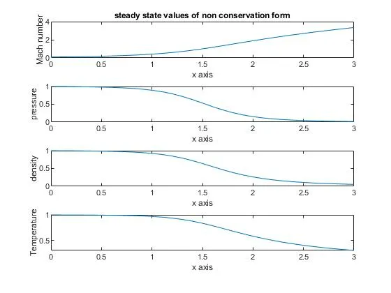
Steady-state distribution of primitive variables inside the nozzle
Non-conservative form
conservative form
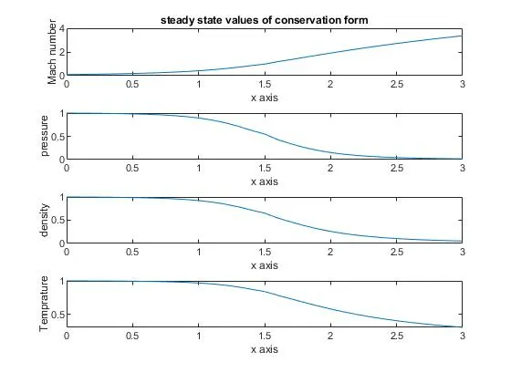
We can see from the graph that the steady-state values are the same for the conservative and non-conservative forms. The curve we are getting for Mach number, Pressure, Density, and Temperature are the same for both conditions. So we get the same values at the steady-state condition either we use non-conservation or conservation form.
Case-2
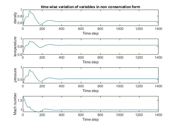
Time-wise variation of the primitive variables
Non-conservative form
conservative form
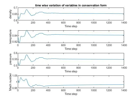
So we can see from both graphs that the values at different time steps are different in the conservative and non-conservative forms. Variation is more in the non-conservative form. Variation in the sense that the range of the Mach number, Pressure, Temperature, and Density values. So when we use the conservation form the values we get are nearer to the steady-state values as compare to the non-conservative form.
With the increase of the time step, it goes to the steady-state condition. When we get to the steady-state condition, we get the same result in both form.
Case-3
Variation of Mass flow rate distribution inside the nozzle at different time steps during the time-marching process
Non-conservative form
conservative form
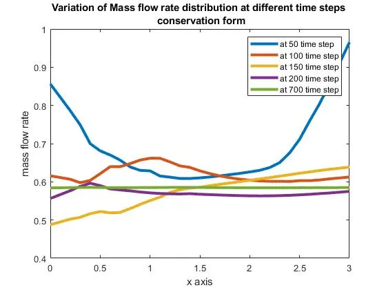
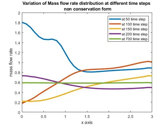
We have taken the mass flow rate at the throat. We can see from both graphs that in conservative form the mass flow rate is much closer to being a constant as compared to the non-conservative form. The mass flow variation is more in the non-conservative form. The range for the non-conservative is 0.1 to 1.8 and in the conservative, the range is from 0.45 to 0.85. So we can say that the mass flow rate is more efficient in the conservative form.
Case-4
Residual inside the nozzle at different time steps during the time-marching process
Non-conservative form
conservative form
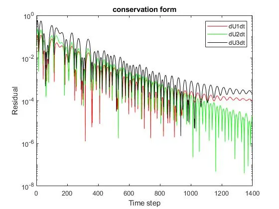
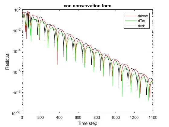
The residual graphs show that the result is converged as the time step increases the error becomes less. In the non-conservative form, it goes below the 1e-6 and in the conservative form, it goes below the 1e-4. So we can say from the graph that the error becomes much less fastly in the non-conservative form as compared to the conservative form.
The non-conservative form leads to a smaller residual as compare to the conservative form.
Case-5
Comparison of Normalized mass flow rate distributions of both forms
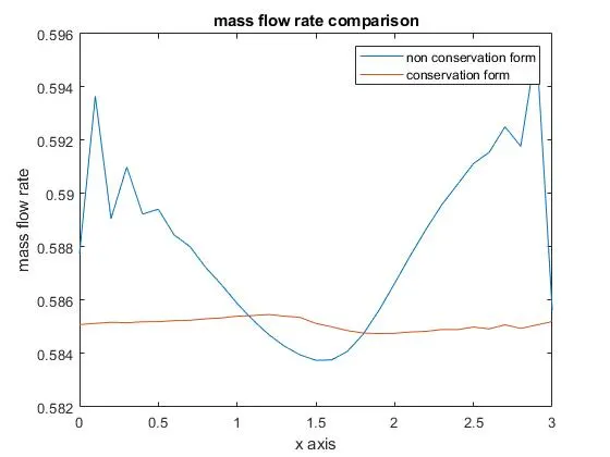
We have taken the mass flow rate at the throat. We can see from both graphs that in conservative form the mass flow rate is much closer to being a constant as compared to the non-conservative form. The steady-state mass flow rate results are much closer to the exact analytical solution.
Grid Independence
Grid independence is when the result values do not change with the change in the number of grid points. We are comparing the values at the throat point and with the analytical values.
| Flow variables | Analytical Solution | Non-conservative form(31 grid points) | Non-conservative form(61 grid points) | Conservative form(31 grid points) | Conservative form(61 grid points) |
| Density | 0.634 | 0.6387 | 0.6377 | 0.6524 | 0.6390 |
| Mach number | 1.000 | 0.9994 | 0.9998 | 0.9780 | 0.9978 |
| Temperature | 0.833 | 0.8365 | 0.8354 | 0.8411 | 0.8357 |
| Pressure | 0.528 | 0.5342 | 0.5327 | 0.5487 | 0.5340 |
So from the above table, we can see that when we compare the analytical solution with the numerical solution, the non-conservative form with 61 grid points gives the more accurate values compare to others. we can see that at the different grid points the values are almost the same(slightly different) so the solution is grid independence.