Simulating fluid sloshing effect inside a gearbox

OBJECTIVE

The primary objective of this challenge is to simulate the 'sloshing' of the fluid inside a gearbox. This challenge is to be carried out in Fluent using the Volume of Fluid method with help of User-Defined Functions (UDF) that generates moving mesh in the gearbox.

GEOMETRY AND PHYSICAL MODEL

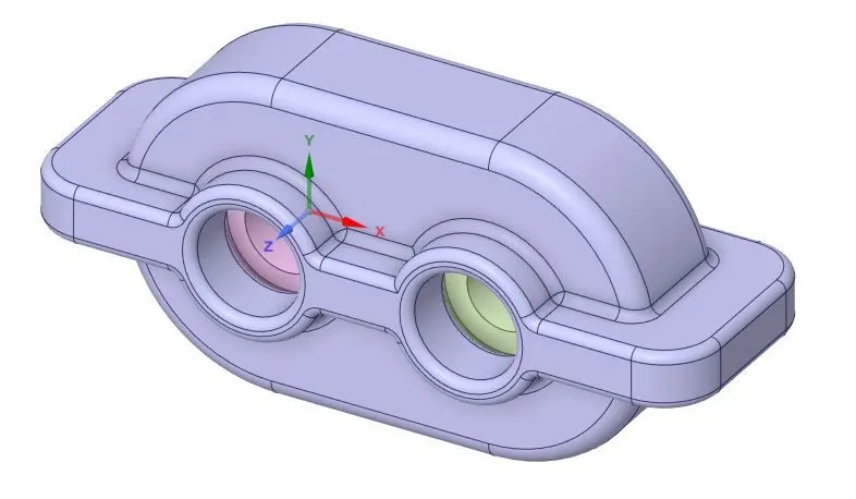
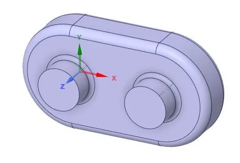
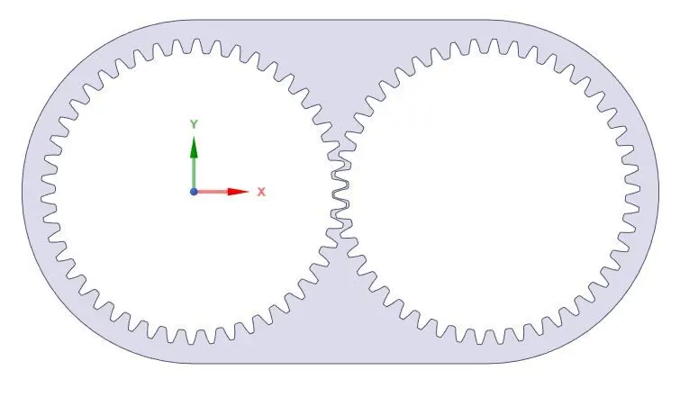
Shown below is the image of the Gearbox. The gearbox consists of two spur gears in a housing. The gearbox is to be filled with a liquid up to a certain height measured as a percentage of the height of the Gearbox. The gears would then be immersed in the liquid up to this height. The gears are run at 200 radians per second. When the gearset is running, this liquid is carried by the teeth that result in self-lubrication of the gearbox. Liquid sloshing also occurs as the result. A complete 3D simulation of the gearbox would be computationally expensive in terms of the mesh and time taken. Hence a 2D simulation is conducted. A transient simulation is performed to capture two complete rotations of the gear. At industry standards, gearbox simulations would be run typically up to 6-7 rotations but, these types of simulations are extremely costly in terms of computational resources.

Four cases are simulated:

1. 20% Immersion, Fluid used - Engine oil
2. 30% Immersion, Fluid used - Engine oil
3. 20% Immersion, Fluid used - n-heptane (C7H16)
4. 30% Immersion, Fluid used - n-heptane (C7H16)

THEORY

i) Liquid Sloshing and its effects:

Liquid Slosh refers to the movement of the liquid inside another object due to an external forcing onto the object or due to internal forcing such as a gear. The liquid must have a free surface to constitute a slosh dynamics problem, where the dynamics of the liquid can interact with the container to alter the system dynamics significantly. Sloshing has negative effects in the case of a container containing liquid. It can result in structural damage to the walls of the object due to the hammering effect of the liquid in repeated intervals. Sloshing can be hazardous during the transport of reacting chemical liquids. To prevent sloshing in containers, Baffles are used. Baffles are essentially walls that reduce the effective free surface elevation attained by the liquid during sloshing. It is also experimentally observed that with an increase in the viscosity of the fluid, the damping effect on the slosh increases.

But in the case of a gearbox, the liquid sloshing has a positive effect. It helps in the complete lubrication of the gear tooth. The lubricant is able to find itself in each and every tooth of the gears.

ii) Theory of Dynamic Meshing in fluent:

The Dynamic Meshing feature in Fluent allows a user to move a particular boundary of a zone rigidly w.r.t. other zones in the boundary. In this case, the dynamic mesh is used on the boundaries of the gear teeth to capture the gear rotation and its effect on the fluid zone. The mesh volume is updated at each timestep by Fluent itself based on the new position of the boundary.

Dynamic meshes can be used in the movement of pistons inside a cylinder, flap deflecting on an aircraft wing, deformation of an elastic wall of a balloon on a rigid surface.

To enable dynamic mesh, the initial mesh and the motion of the boundary are required. The motion of the boundary can be specified by a User-defined function (UDF), by using Boundary Profiles or a 6-DOF Solver. There are three methods of dynamic meshing in Fluent:

a) Smoothing Methods:

In the smoothing method, the nodes of the mesh move, but the number of nodes and connectivity do not change. There are 3 types of smoothing methods: i) Spring-based, ii) Diffusion, iii) Linearly elastic solid

In the spring-based method, edges between any two mesh nodes are idealized as a network of inter-connected springs. Displacement of a node will generate a force proportional to displacement along with all springs connected to that node. This method can be applied to the mesh zones that are moving/ deforming. This method is predominantly used for tetrahedral meshes.

The diffusion-based method is used for polyhedral meshes. It is computationally more expensive but yields higher quality results compared to the spring-based method. This method allows larger boundary deformations before breaking down and can handle rotational motions. The linearly elastic solid is more accurate than the diffusion method.

b) Dynamic Layering:

Dynamic Layering is used to split/ merge cells adjacent to a moving boundary when the following conditions are met.

• Cells adjacent to moving boundary are wedges or hexahedrons (quadrilaterals in 2D)
• Cell zones must be completely bounded by one-sided face zones.

c) Remeshing:

When the boundary displacement is very large compared to cell sizes, cell quality may deteriorate if only mesh smoothing is used. To avoid this, Fluent can agglomerate cells or faces. If the new cells satisfy the imposed skewness criterion, the old cells are replaced by the new cells. Otherwise, the old cells are retained. Fluent offers 5 re-meshing methods. In this challenge, the Local Cell Re-meshing method is used.

In Local Cell Remeshing, Fluent agglomerates cells based on skewness, size, and height prior to movement of the body. The size criteria are the Minimum and Maximum length scales. The desired skewness is also entered by the user. Cells that are below the minimum length scale and greater than the maximum length scale are marked for re-meshing. Marking based on skewness is done every timestep and marking based on the size is done based on the specified time interval.

iii) Volume of Fluid Method:

The Volume of Fluid (VOF) model is a surface tracking method that finds the interface of two or more immiscible liquids. The phases in each cell of the mesh are known by the Volume Fraction of the cell. The equations involved in the VOF modeling are the i) Volume fraction equation, ii) Momentum equation iii) Energy equation.

The volume fraction equation is basically the solution of the continuity equation for each phase and its solution gives the volume fraction of the phase. The sum of volume fraction of all phases in a cell must be equal to 1. Both explicit schemes and implicit schemes are used to solve the volume fraction equation. The transient formulation is used for both steady and transient states. The explicit formulation is used for transient states only. Shown below is the volume fraction equation for a phase 'q'. Here 'p' represents another phase.

The Momentum and the Energy equation are shared by all the phases. The density and viscosity of the phases in a cell influence the resulting velocity.

iv) The use of User Defined Function (UDF) in this challenge:

The gearbox contains gears that are in rotation. Hence this movement will affect the dynamics of the liquid present. To capture this, the dynamic mesh needs to be enabled. The inputs to the dynamic mesh are the initial mesh and the boundary motion.

In the meshing module, the initial mesh is generated with the all triangles method. Two named selections representing the moving boundary of the fluid domain are created. The boundary motion of this named selection is specified by a User Defined Function (UDF). The UDF code is shown below.

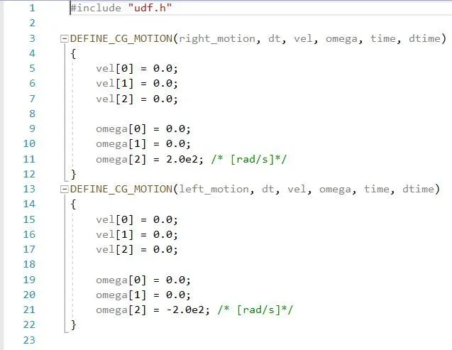
DEFINE_CG_MOTION is a function under the library of 'udf.h' which enables rotation of dynamic zones within a center of gravity. Its arguments are given by 'DEFINE_CG_MOTION (name, dt, vel, omega, time, dtime)', where name is the name of UDF, dt is a pointer to a structured dynamic data, vel is the linear velocity provided to dynamic mesh zone, omega is the rotational velocity provided to dynamic mesh zone, time is the time at which the particular speed can be specified, dtime is the timestep.

The right gear motion is specified first. vel[0] = vel[1] = vel[2] = 0 indicate that linear velocity of the dynamic zone is zero along the X, Y, Z axes. omega[1] = 0, omega[1] = 0, omega[1] = 200 indicate that rotational velocity of the dynamic zone is zero along the X, Y axes and is 200 rad/sec on the Z-axis. Similar codes are written for the other gear. This UDF will enable the rotation of the gears in the opposite direction.

v) Common errors faced in the user's simulation:

i) 'Negative cell volume detected' error:

During dynamic meshing, if the displacement of the boundary is more than the local cell size, it can deteriorate the quality of cells (skewness). This will lead to negative cell volume.

ii) 'Floating Point' error:

The floating-point error occurs when the solver detects an expression that cannot be solved by numerical methods. These kinds of expressions often lead to divergence of the solution. The problems using the volume of the fluid method are susceptible to large time steps especially at initial iterations where the velocity of flow is still very low. Upwind schemes can be used for discretization. They introduce numerical diffusion but ensure convergence. Higher-order schemes are not to be used. Under-relaxation methods are an effective way to avoid floating-point errors.

CASE SETUP IN ANSYS:

I) Geometry:

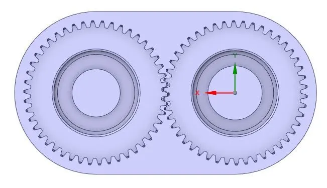
A 2D fluid volume domain is extracted from the 3D geometry. The series of steps are as followed are shown: 3D geometry ==> Extract fluid volume using 'Volume Extract' command ==> 'Split Body' command to obtain half body ==> fluid surface that contains the boundary of gear copied and pasted in a new window.

II) Meshing:

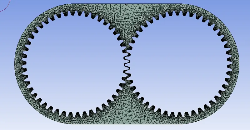
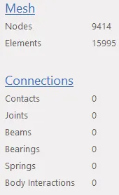
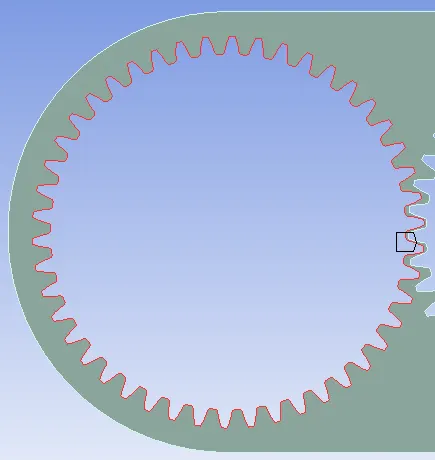
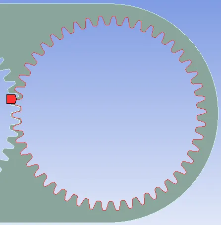
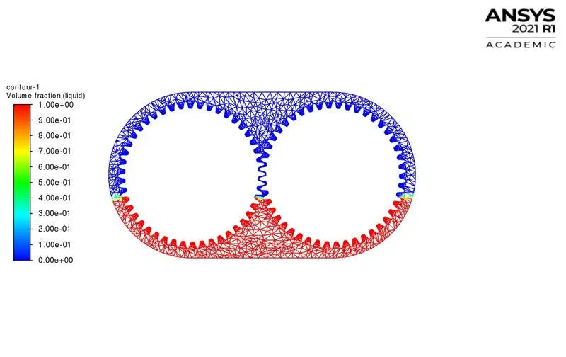
The meshing method is set to 'All triangles'. The initial mesh element size is set to 30 mm. 'Capture proximity' is enabled with the number of cells across the gap set to 1. A total of 15995 elements are created in this mesh which is reasonable for a 2D simulation. Next, edge-named selections 'gear_left' and 'gear_right' are created at the boundaries of the gear. This is done in order to specify the motion of the boundaries with a UDF in Fluent.

III) Fluent set-up:

• A pressure-based, transient solver is used. Gravity is enabled with -9.81 m/s^2 in the Y direction.
• The Realizable k-ε">k−ε�-� with an Enhanced wall treatment turbulence model is selected.
• The Volume of Fluid method is enabled under the Multiphase tab with two Eulerian phases. Phase 1 is selected as 'air'. Phase two is selected as 'Engine-oil' or 'N-heptane'. The implicit formulation is selected for the solution of the Volume fraction equation.

• The SIMPLE solver is chosen for the pressure-velocity coupling. Since this is a VOF simulation, higher-order discretization is not used. In addition, stricter under-relaxation factors are provided to avoid the Divergence of the solution.
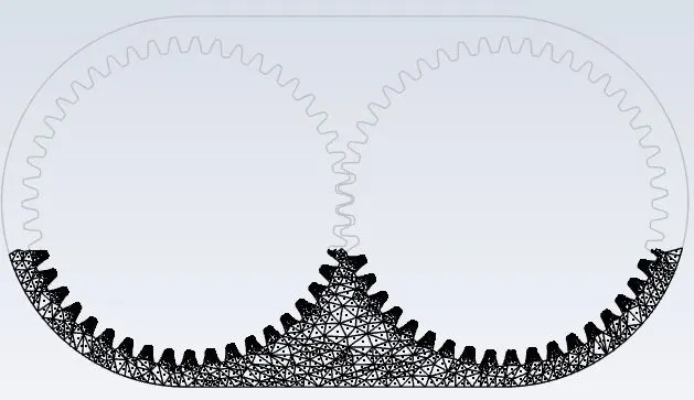
• To make a part of the fluid domain to be occupied by Phase 2, these cells have to be marked. This is done using Refine/coarsen option under the Domain tab.
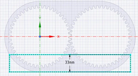
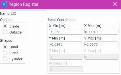
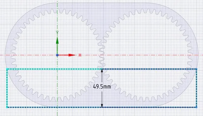
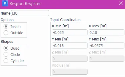
• In the refine/coarsen option, the coordinates of the diagonal a 'quad' region whose area covers the fluid domain up to 20% or 30% immersion of the gearbox are specified. These coordinates are obtained from SpaceClaim where a dummy rectangle is sketched with a height of the corresponding immersion level. The marked region and the coordinates are shown for both the 20% immersion and 30% immersion.
• 20% Immersion ==> 20% of ht of gearbox ==> 0.2 X 165 mm = 33 mm. The region is marked for patching.

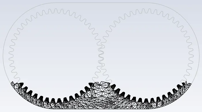
• 30% Immersion ==> 30% of ht of gearbox ==> 0.3 X 165 mm = 49.5 mm. The region is marked for patching.

• Next, the UDF is to be loaded. To load the UDF, under User-defined tab, Functions ==> Compiled UDF's ==> Add rate.C (filename of UDF) ==> Click 'Build' ==> Click 'Load'. The UDF file which is shown above is loaded. The UDF specifies the motion of the boundary of the gear. They are named as right_motion and left_motion.
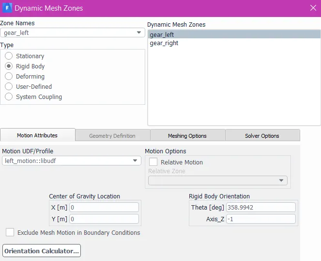
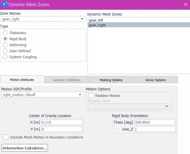
• Next, the dynamic mesh is to be set up. The motion is set to the zones which were created by the named selections during Meshing. The motion profile is available from the UDF as a drop-down box which consists of right_motion::libudf and left_motion::libudf. The centers of gravity of the gears are specified along with the motion.

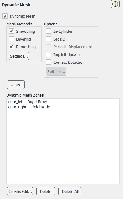
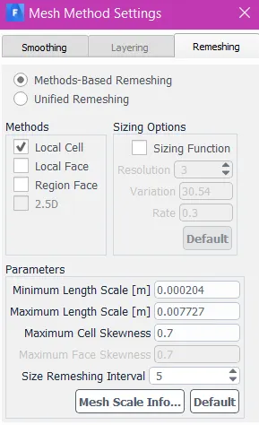
• Dynamic mesh method 'Smoothing' and 'Remeshing' is enabled. The Smoothing method is set to 'Diffusion based'. The Remeshing methods and parameters are shown below. These remeshing parameters based on size are automatically suggested by Fluent based on the initial mesh. It is modified if Negative Cell Volume Error arises and as per the quality of mesh required. With this, the dynamic mesh is set up.

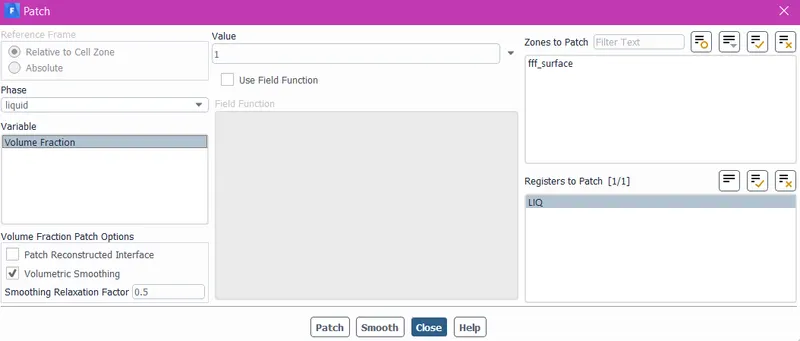
• Finally, the simulation is initialized with a hybrid solver. The marked region is then patched with the corresponding Phase 2. The contour of the Volume Fraction of Phase 2 is set up. Solution animation of the Volume fraction contour is also set up to observe the sloshing and the lubrication that occurs.

• The timestep size is chosen as 1e-5 sec after trial and error. Timestep size of 1e-4 sec and above led to floating-point error. It is important to choose a small timestep size in order to avoid the floating-point error that arises due to divergence. The number of time steps is calculated as follows.
• Speed of rotation of gear = 200 rad/ sec = 31.83 RPS; ==> 1 rotation = 31.83^-1 sec = 0.0314 sec. ==> 2 rotations = 0.0624 sec.
• Number of timesteps required = 0.0624 sec / 1e-5 sec = 6240. Hence, the number of timesteps is specified as 6300.
• The solution is then calculated for the 4 mentioned cases.

RESULTS:

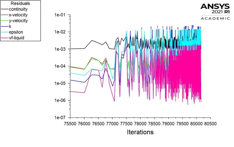
1) Convergence:

Case #1: 20% Immersion-Engine Oil

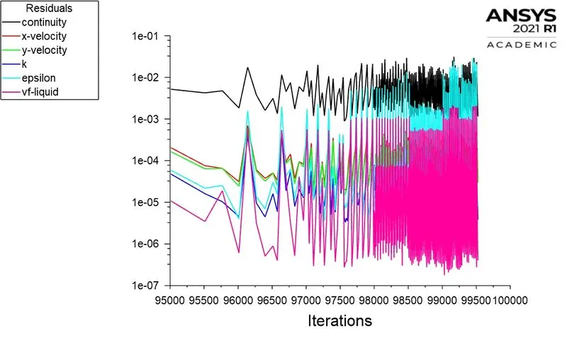
Case #2: 30% Immersion- Engine Oil

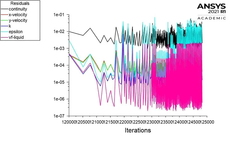
Case #3: 20% Immersion-N Heptane

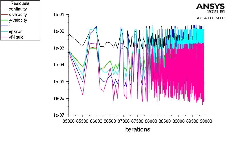
Case #4: 30% Immersion-N Heptane

2) Volume fraction plots and Animations:

Case #1: 20% Immersion-Engine Oil

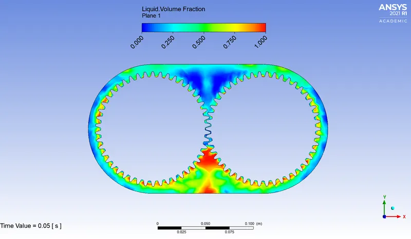
Case #2: 30% Immersion- Engine Oil

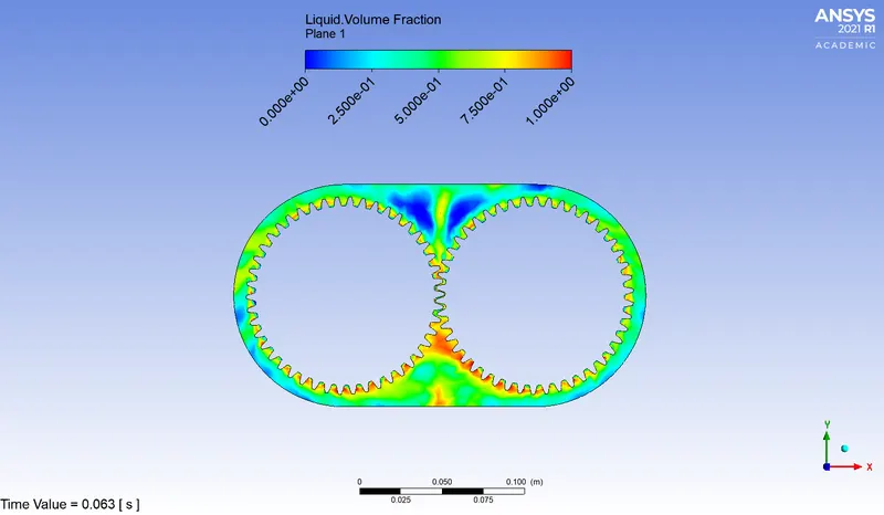
Case #3: 20% Immersion-N Heptane

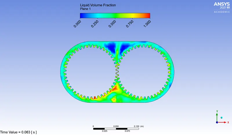
Case #4: 30% Immersion-N Heptane

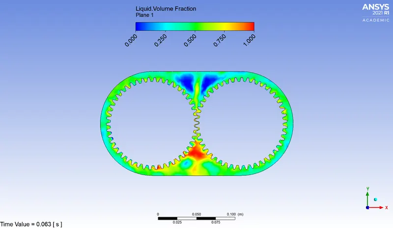
• As the gear starts to rotate, it carries the lubricant with itself.
• After one rotation of the gear, at the region where the gears mesh, the is an upward throw of the lubricant which hits the top walls of the gearbox resulting in sloshing.
• Due to the viscosity of the lubricant and primarily the velocity at which it gets thrown from the gear mesh, the lubricant travels a short distance along the wall after which it falls back on the gears moving in the opposite direction of gear motion.
• In the course of rotation of the gear, it is noticed that some lubricant slips from the gears and falls back into the pool.
• It can be eventually realized that, as the gears move in forward rotation, the lubricant moves in backward rotation. The lubricant slips through the teeth, falls onto the pool, moves towards the region of gear mesh, and gets thrown and sloshed.
• Sloshing accelerates the lubricating action. Eventually, the lubricant reaches all the teeth and the gears get completely lubricated.
• With an increase in immersion level from 20% to 30%, the gearbox gets lubricated faster. The lubricant reaches all of the significant parts of the fluid domain in lesser time. This is observed in both the lubricants.
• Engine oil is more viscous than n-heptane. From the animation, it is observed that the slip that occurs when the lubricant is transported is significantly lesser for the engine oil. The backward slip velocity of the lubricant is much lesser.
• The engine oil that gets sloshed sticks to the wall due to its higher viscosity. It is also observed that the engine oil deposits on the teeth on an account of its higher viscosity.

CONCLUSION

Liquid Sloshing and its effect on lubrication are simulated in a gearbox. Four simulations are conducted with varying immersion levels and lubricating material. With the increase in the immersion level, lubrication occurs faster. With the increase in the viscosity of the lubricant used, the lubricant sticks with the walls and surfaces.

The Volume of Fluid multiphase method is used along with a dynamic mesh in this challenge. A smaller timestep may lead to better convergence. Remeshing with modified size-based parameters is used to avoid negative cell volume error.