Project

SI Engine Performance Characteristics Using MATLAB

RRoshan Shaik8 Sept 2021

Engine performance is an indication of the degree of success with which it does its assigned job i.e., conversion of chemical energy contained in the fuel into useful mechanical work.

AIM

To evaluate the performance characteristics of a SI engine using MATLAB.

OBJECTIVE

To perform the below tests on a 2005 Triumph Tiger 955i engine:

To Graphically represent the fuel map of the selected SI engine
To plot the fuel consumption rate curves
To plot the power V/S Engine speed curves
To plot the mean effective pressure V/S Engine speed curve
To plot the Specific fuel consumption V/S Brake mean effective pressure curve
To calculate the Thermal efficiency of the engine
To calculate the brake thermal efficiency of the engine
To calculate the specific output of the selected engine

SIGNIFICANCE OF THE PROJECT

Computational engine performance refers to how the engine performs in terms of power produced, torque produced, mechanical and thermal efficiencies. This type of computational engine performance tests can act as a pre-step to actual real world testing of the engine - this would cut down the R&D costs of developing a vehicle. This would also allow the designer to randomly generate various combinations of bore x stroke lengths for the same displacement to see how it reacts without designing the engine in the first place.

This computational engine testing can be included in the domain of Computer Aided Engineering of Automobiles.

It also provides a good start to beginning to design an engine, like which we can get the approximate values so, iteration times are reduced and development time decreases and improves accuracy.

THEORY

Basic Terms of IC engines:

Swept Volume:

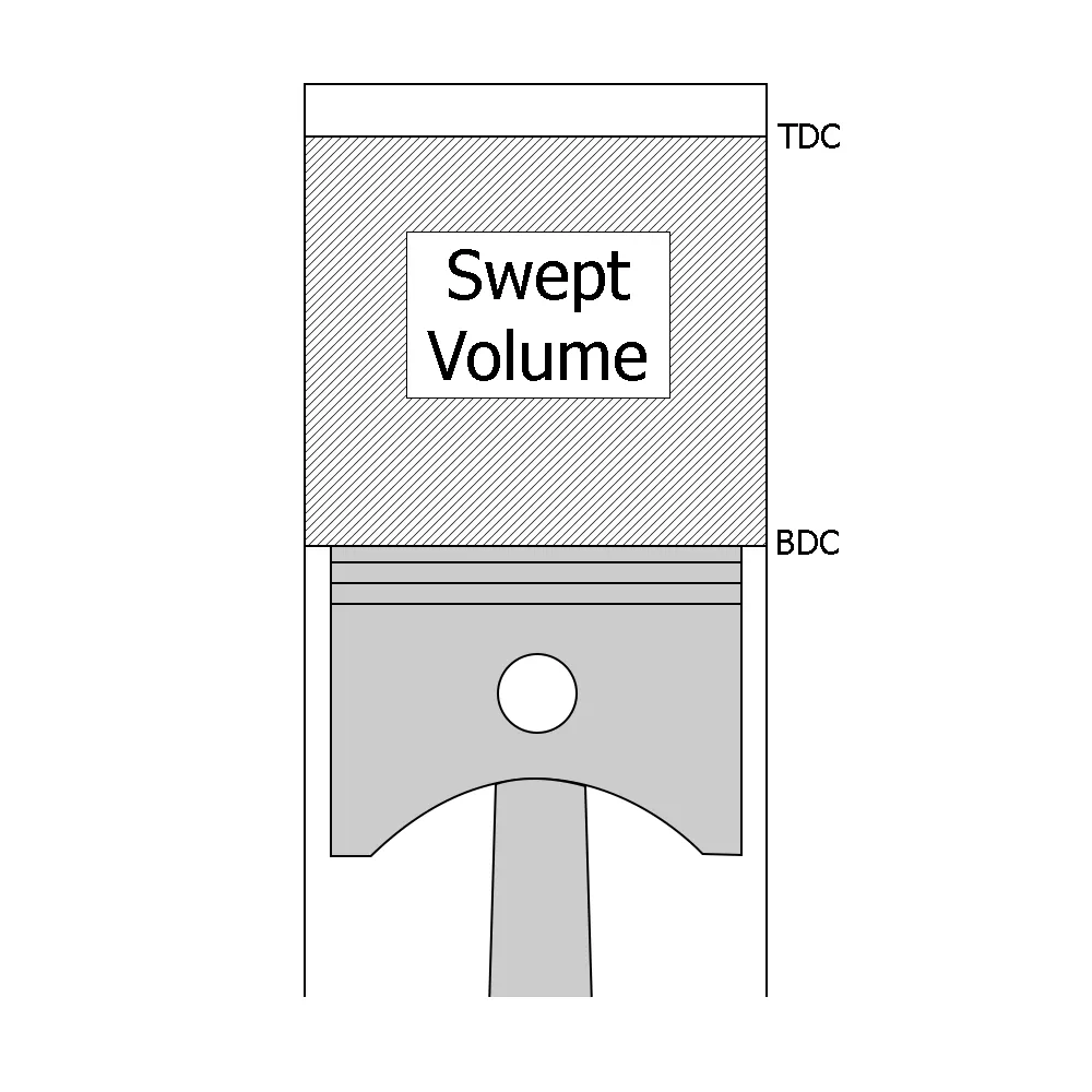
The volume swept through by the position in moving from the top dead centre (TDC) and bottom dead centre (BDC), is called the piston displacement or swept volume.

Thus, when the piston is at BDC,

Swept Volume, `V_s = n*A_p*L`

Where,

`A_p`, Area of piston, `A_p = pi/4*D_b^2`

`D_b`, Bore diameter: Diameter of the piston face

`L`, Stroke length: Length between TDC and BDC

2. Engine Displacement

The total displacement of the engine.

`V = n*V_s`

where,

`n`, Number of cylinders

3. Clearance volume:

The volume left inside the cylinder when the piston is at the TDC e., the volume between cylinder head and piston at TDC is called Clearance volume.

Clearance volume, `V_c = V_s/(gamma – 1)`

Where,

`gamma` is the adiabatic constant: `C_p/C_v`

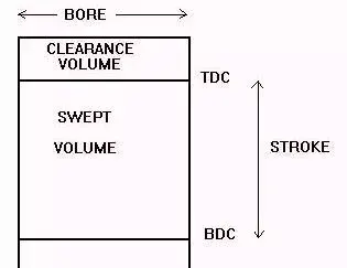
4. Compression ratio: It is the ratio of total swept volume to the clearance volume.

Compression ratio, `r_c = V_s/V_c`

Fuel consumption

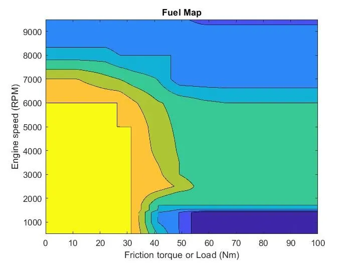
For a dynamic system, the fuel consumption varies with varying speed and load on the engine. This is so because the fuel consumption is dependent on the air-fuel ratio, for which the engine has a predefined map called "Fuel map" which defines the fueling character of the engine.

mass of fuel = (mass of air in the engine cylinder at BDC)/air-fuel ratio.

The mass flow rate of fuel = mass of fuel*Engine speed.

Fuel map

A fuel map is the combination of everything an ECU knows about engine running conditions. The goal of a fuel map is to use this information to provide the right amount of fuel. It does this by controlling fuel injector pulse width. Pulse width (PW) is the amount of time an injector is open in milliseconds.

Example of a fuel map configurator.

Otto-cycle:

Please refer to the below project for more info on simulating the Otto cycle.

https://skill-lync.com/projects/thermal-efficiency-and-pv-plots-of-an-air-standard-otto-cycle

Combustion temperature (`T3`)

Although the above project uses a constant value of combustion temperature `T_3`, with varying air-fuel ratios it is subject to change.

`T_3` is a function of the mass flow rate of fuel.

`T_3 = T_2 + (LHV*m_f*C_p)`

Where,

`T_2` is the temperature inside the combustion chamber at the end of the compression stroke.

`LHV` is the Lower calorific value of the fuel

`m_f` is the mass flow rate of the fuel

`C_p` is the specific heat of fuel at constant pressure

2. Work Done

The net work done per kg in the Otto cycle by the engine can be calculated by using the values of pressure and volume.

`W = (V_1/(gamma - 1))*[(r^(gamma - 1) - 1)*(P_4 – P_1)]`

Where,

`V_1 = V_s – V_c`

`r = V_s/V_c` : Compression ratio

3. Mean Effective Pressure

The mean effective pressure is defined as a hypothetical pressure that is thought to be acting on the piston throughout the power stroke.

`P_(me) = W/V_s`

The most accurate theoretical mean effective pressure can be acquired from the mean of pressure trace of the otto cycle during the expansion stroke.

Engine Performance

Engine performance is an indication of the degree of success with which it does its assigned job i.e., conversion of chemical energy contained in the fuel into useful mechanical work.

Indicated Power

The total power developed by the combustion of fuel in the combustion chamber is called indicated power.

Indicated power, IP = `(n*P_(me)*Stroke*A_p*k*10)/6` kW

where,

`P_(me)` is the indicated mean effective pressure

k = 0.5 for a 4-stroke engine and 1 for 2-stroke engine

Brake Power

The power developed by an engine at the output shaft is called the brake power.

Brake power, BP = `(2*pi*N*T)/60`

where,

T is the torque.

But since the Engine torque is unknown, we will utilize the mechanical efficiency to calculate the Brake power.

Then,

BP = IP * Mechanical Efficiency

Friction Power

It is the difference between Indicated power and Brake power.

FP = IP - BP

Specific Output

It is defined as the brake output per unit of piston displacement. It is given by,

Specific Output = `(BP)/(A_P*L)`

Specific Fuel Consumption

It is the mass of fuel consumed per kW developed per hour and is a criterion of economical power production.

`s.f.c =m_f/(BP)`

Thermal efficiency is the ratio of indicated work done to the energy supplied by the fuel.

Indicated Thermal Efficiency

ITheff = `(IP)/(m_f*LHV)`

Brake Thermal Efficiency

BTheff = `(BP)/(m_f*LHV)`

The MATLAB CODE:

Main code:

close all
clear all
clc

%% 4-stroke single cylinder SI engine specifications

% User inputs
prompt = {"Bore diametre (cm)","Stroke length (cm)","Compression ratio","Connecting rod length (cm)","Number of cylinders","Strokes per cycle","Idle engine speed (RPM)","max engine speed (RPM)","Minimum Load (Nm)","Max Load (Nm)"}; %#ok<*CLARRSTR>
dlgtitle = "SI Engine specification";
dims = [1 50];
definput = {'7.9', '6.5', '11.6', '30', '3', '4','500','9500','0','100'};
inputs = inputdlg(prompt,dlgtitle,dims,definput);
engine_specs = str2double(inputs);

    bore = engine_specs(1); % Diametre of bore in cm
    stroke = engine_specs(2); % Length of stroke in cm
    rc = engine_specs(3); % Compression ratio of the engine
    cont_rod = engine_specs(4); % Connecting rod length in cm
    n = engine_specs(5); % Number of cylinders
    z = engine_specs(6); % Number of strokes
    N_idle = engine_specs(7); % Engine idling speed
    N_max = engine_specs(8); % Engine max speed
    Tf_min = engine_specs(9); % Minimum loan in Nm
    Tf_max = engine_specs(10); % Maximum Load in Nm
    clear engine_specs
    
        area_piston = pi*(bore/2)^2; % Area of piston face 
        Vds = area_piston*stroke; % Displacement of the engine in cc
        Vd = n*Vds; % Total displacement of the engine in cc
        
        if z == 4
            k = 0.5; % For 4 stroke engines
            m = 2;
        else
            k = 1; % For 2 stroke engines
            m = 1;
        end

%% Reading the fuel map

prompt = "Enter the name of the file containing the fuel map";
name_of_file = char(inputdlg(prompt));

file = readtable(name_of_file);
clear name_of_file

% Sorting the varibles for the tabel
fuel_map = file(2:17,2:17); 
    fuel_map = table2array(fuel_map);
load = file(2:17,1:1);
    load = table2array(load); 
engine_speed = file(1:1,2:17);
    engine_speed = table2array(engine_speed);
    
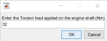
prompt = "Enter the Torsion load applied on the engine shaft (Nm)";
net_Tf = str2double(inputdlg(prompt));

%% Fuel specs
% User inputs
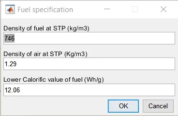
prompt = {"Density of fuel at STP (kg/m3)","Density of air at STP (Kg/m3)","Lower Calorific value of fuel (Wh/g)"};
dlgtitle = "Fuel specification";
dims = [1 50];
definput = {'746','1.29','12.06'};
inputs = inputdlg(prompt,dlgtitle,dims,definput);
fuel_specs = str2double(inputs);

    dens_fuel = fuel_specs(1);
    dens_air = fuel_specs(2);
    LHV_fuel = fuel_specs(3);
    clear fuel_specs
    
%% Otto cycle

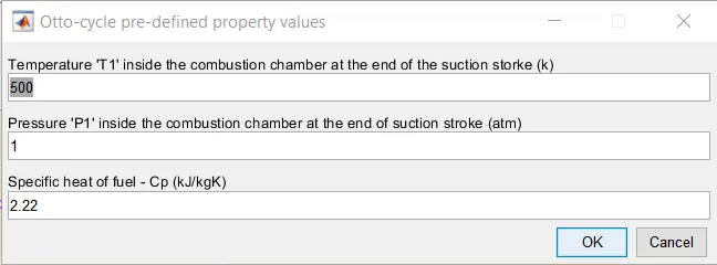
prompt = {"Temperature 'T1' inside the combustion chamber at the end of the suction storke (k)","Pressure 'P1' inside the combustion chamber at the end of suction stroke (atm)","Specific heat of fuel - Cp (kJ/kgK)"};
dlgtitle = "Otto-cycle pre-defined property values";
dims = [1 90];
definput = {'500','1','2.22'};
inputs = inputdlg(prompt,dlgtitle,dims,definput);
otto_propts = str2double(inputs);

    T1 = otto_propts(1);
    P1 = otto_propts(2)*1.013;
    Cp = otto_propts(3);
    clear otto_propts
    
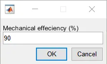
prompt = "Mechanical effeciency (%)";
input = inputdlg(prompt);
engine_perf = str2double(input);

mech_eff = engine_perf/100;
    
%% Fuel map 

afr = zeros();
N = linspace(N_idle,N_max,N_max-N_idle); 
Tf = linspace(Tf_min,Tf_max,Tf_max-Tf_min);
for i = 1:length(N)
    for j = 1:length(Tf)
        afr(i,j) = interp2(engine_speed,load,fuel_map,N(i),Tf(j));
    end
end

%% Engine fueling 

afr_net = zeros(); m_fuel = zeros(); mf = zeros(); vf = zeros();
m_air = dens_air*(10^-3) * Vds; % Mass of air in g
for i = 1:length(N)
    afr_net(i) = interp2(engine_speed,load,fuel_map,N(i),net_Tf);
    m_fuel(i) = m_air/afr_net(i); % Mass of fuel consumed per cycle per cylinder
    
    mf(i) = n*m_fuel(i)*N(i)/(m*60); % Mass flow rate of fuel per second in g/s
    vf(i) = mf(i)/(dens_fuel/1000); % Volume flow rate of fuel per second in g/s
end

%% Otto cycle of 1 cylinder
 % Requred inputs: Vds, T1, P1, rc, LHV_fuel, mf
 
    % Requisite calculations
        y = 1.4;
        Vcs = Vds/(rc-1); % Clearance volume
        
    % State 1
        V1 = Vds + Vcs;
        
    % State 2
        V2 = Vcs;
        P2 = P1*rc^y;
        T2 = T1*rc^(y-1);
    
    % State 3
        V3 = Vcs;
        V4 = V1;
        T3 = zeros(); P3 = zeros(); P4 = zeros(); T4 = zeros(); W = zeros(); Pm = zeros(); c = zeros(); p_mi = zeros();
        for i = 1:length(N)
                T3(i) = (LHV_fuel*m_fuel(i)*Cp)+T2;
                P3(i) = P2*T3(i)/T2;

            % State 4
                P4(i) = P3(i)*(rc^-y);
                T4(i) = T3(i)*rc^(1-y);

            % Work Done
                W(i) = n * V1 * ((rc^(y-1))-1)*(P4(i)-P1)/(y-1);

            % Mean effective pressure 
                Pm(i) = W(i)/(V1 - V2);
                
            % Piston kinematics for icentropic expansion process
            c(i) = P3(i)*V3^y;
            v_expansion = engine_kinematics(stroke,cont_rod,rc,0,180,Vcs/n);
            p_expansion = c(i)./v_expansion.^y;
           
            p_mi(i) = (sum(p_expansion,'all')/length(p_expansion)); % Indicated mean effective pressure (bar)
            
        end
        
    % Thermal effeciency
        TE = 1 - rc^(1-y); 

%% Engine performance (Static)

IP = zeros(); BP = zeros(); FP = zeros(); SO = zeros(); sfc = zeros();
for i = 1:length(N)
    IP(i) = p_mi(i)*(stroke/100)*(area_piston*10^-4)*N(i)*k*10/6; % Indicated power (kW)
    BP(i) = IP(i)*mech_eff; % Brake power (kw)
    FP(i) = IP(i)-BP(i); % Frictional power losses (kw)
    
    SO(i) = BP(i)/1000*n*Vds; % Specific output (W/cc)
    sfc(i) = mf(i)*3600/(1000*BP(i)); % Specific fuel consumption (g/kWh)
end

SO_avg = (sum(SO,'all')/length(SO));
j = randsample(length(N),1);
ITheff = IP(j)/(LHV_fuel*mf(j)); % Indicated thermal effeciency
BTheff = BP(j)/(LHV_fuel*mf(j)); % Brake thermal effeciency
        
%% Plotting 

% Fuel map plot
figure()
grid on
contourf(Tf,N,afr)
title('Fuel Map')
ylabel('Engine speed (RPM)')
xlabel('Friction torque or Load (Nm)')
colormap default

% Engine fueling for specific load
figure()
grid on
hold on
plot(mf*60,N)
plot(vf*60,N)
title('Flow rate of fuel VS Engine speed')
xlabel('Flow rate of fuel')
ylabel('Engine speed (RPM)')
legend('Mass flow rate (g/min)','Volume flow rate (cc/min)')

% Engine speed V/S Mean effective pressure
figure()
grid on
plot(N,p_mi)
title('Bmep VS N')
xlabel('Engine Speed (RPM)')
ylabel('Mean effective pressure (bar)')

% Power V/S Speed
figure()
grid on
hold on 
plot(N,IP)
plot(N,BP)
plot(N,FP)
title('Power VS Speed')
xlabel('Engine speed (RPM)')
ylabel('Power (kW)')
legend('Indicated power','Break power','Friction power')

% SFC VS Bmep
figure()
grid on
plot(p_mi,sfc)
title('Specific fuel consumption V/S Brake mean effective pressure curve for SI engine')
xlabel('Brake mean effective pressure (bar)')
ylabel('Specific fuel consumption (g/kWh)')

% Specific output
figure()
grid on
plot(linspace(0,Vd,length(SO)),SO)
title('Specific Output VS Volume')
ylabel('Specific output (W/cc)')
xlabel('Volume (cc)')

%% Output 
fprintf('Bike make: 2005 Triumph Tiger 955in');
fprintf('Bore x Stroke: %f mm x %f mmn',bore,stroke);
fprintf('Number of cylinders: %fn',n);
fprintf('%d strokesn',z);
fprintf('Mechanical efficiency %fn',TE*100);
fprintf('n');
fprintf('The total displacement of the engine is %f ccn',Vd);
fprintf('The thermal effeciency of the engine is %fn',TE*100);
fprintf('The Brake thermal effeciency of the engine is %fn',BTheff*100);
fprintf('The engine produces a brake power of %f kW at %f RPMn',BP(end),N(end));
fprintf('The average specific output of the engine is %f W/ccn',SO_avg);

%% Optimization 

clear prompt digtitle dims definput inputs file i j

Function code:

Engine kinematics

function [V] = engine_kinematics(stroke,cont_rod,cr,start_crank,end_crank,clear_vol)
    % Start_crank is the angualar position of flywheel when the piston is at the top dead centre
    % End_crank is the angular position of flywheel when the piston is at
    % the bottom dead centre
    theta = linspace(start_crank,end_crank,180); 
    
    R = 2*cont_rod/stroke; % Assembly height
    
    % Calculation of the Volume trace
    term1 = 0.5*(cr-1);
    term2 = R + 1 - cosd(theta);
    term3 = (R^2 - sind(theta).^2).^0.5;
    V = (1 + term1*(term2 - term3)).*clear_vol; % Volume trace in cc
end

CODE EXPLANATION:

MAIN CODE:

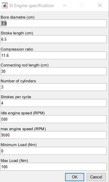
Line 7:25 - Gathering the inputs of the engine specification from the user using a dialogue prompt.

Bore, stroke, compression ratio, connecting rod length, engine speed, engine strokes, idle speed, max speed, minimum load and max load are collected and put into their respective variables.

Line 27:37 - Calculating Engine displacement.

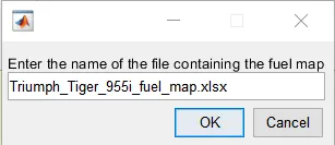
Line 41:53 - Reading the fuel map from an excel sheet

Reading a table in the excel sheet using the readtable() function

1st column is read as the load on the engine and the 1st row is read as the Engine speed.
Everything in between is considered a mesh grid of x and y, which is the air-fuel ratio and is equal to z.

Line 56 - User-defined load torque is read from the user using the inputdlg() function.

Line 60:96 - Specification of the fuel used is read from the user

The density of fuel and air and the lower calorific value is collected from the user.

Line 74:88 - Pre-defined values are inputted to run the otto cycle

The temperature T1 should always be less than the auto-ignition temperature of the fuel
The P1 is near to 1 atm during the suction stroke, hence due to the pressure difference between the fuel injector and the cylinder, the air-fuel mixture flows into the combustion chamber
The Cp value of the fuel and the mechanical efficiency of the fuel.

Line 94-101 - Interpolation of the fuel map for every engine speed of the engine from 500 to 9500 RPM and loads 0 to 100 Nm

The intrep2(x,y,z,x1,y1) produces the value of z1 which is the air-fuel ratio at a custom engine speed and load.

Line 105:113 - Calculating the Fuel consumption of the engine for the entire rev range and at a constant torque which was previously defined by the user.

Line 115:158 - Running the Otto cycle to calculate T3 and the piston kinematics to obtain mean pressure at the expansion Storke.

On line 134 a loop of N iteration is started because the values T3 and everything next change with varying air-fuel ratios. So we get N number of values for each variable specific to each engine speed.
In order to calculate the Indicated Mean effective pressure, the average value of pressures at expansion is taken. It also changes for every different air-fuel ratio.
Finally, the thermal efficiency of this otto cycle is calculated. It remains constant for any air-fuel ratio because it only depends on the compression ratio of the engine.

Line 160:175 - Heart of the project, by calculating all the above values, the primary engine performance characteristics are calculated for every engine speed, engine torque and air-fuel ratio.

Indicated power, Braker power, Friction power, Specific output and Specific fuel consumption is calculated for each value.
Overall Specific output of the engine is calculated by taking the average of all specific output values.
Finally, the indicated thermal efficiency and Brake thermal efficiency is calculated.

Line 177:233 - Plotting the performance curves

Fuel map graph, the Flow rate of fuel V/S Engine speed, Brake mean effective pressure V/S Engine speed, Power V/S Engine speed, Mean effective pressure V/S Specific fuel consumption and Specific output V/S Volume are plotted.

Line 235:246 - Printing the calculated values in the command prompt

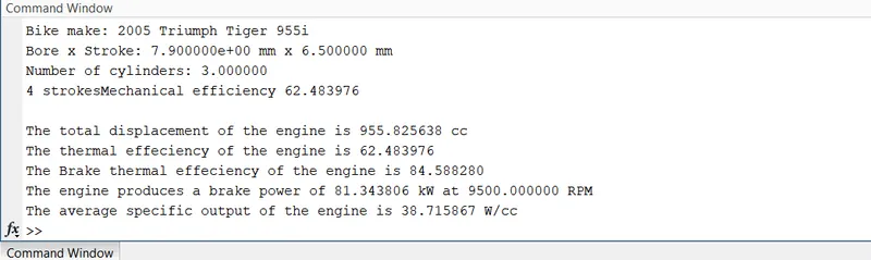
Motorcycle make, Bore*stroke, a number of cylinders, Number of strokes, Mechanical efficiency, Total engine displacement, Thermal efficiency, Brake thermal efficiency, brake power and average specific output of the engine is displayed here.

FUNCTIONS UTILIZED IN THIS CODE:

1. INTREP2:

Vq = interp2(X,Y,V,Xq,Yq) returns interpolated values of a function of two variables at specific query points using linear interpolation. The results always pass through the original sampling of the function. X and Y contain the coordinates of the sample points. V contains the corresponding function values at each sample point. Xq and Yq contain the coordinates of the query points.

OUTPUT:

User inputs:

1. SI Engine specification

2. Name of the file containing the fuel map table

3. Entering the specification of the fuel

4. Entering the Load torque applied on the engine shaft to calculate the fuel consumption

5. Entering the temperate and pressure at state 1 of the otto cycle and the specific heat value of the fuel.

6. Entering the Mechanical efficiency of the engine

RESULTS

1. FUEL MAP

The x-axis represents Friction torque (Nm)
The y-axis represents the Engine speed (RPM)
The x-y plane represents the air-fuel ratio. Each colour represents one air-fuel ratio value. Yellow-green-blue: High-Medium-Low.

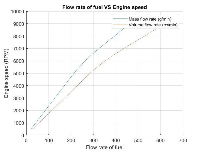
2. FLOW RATE OF FUEL VS ENGINE SPEED AT A SPECIFIC TORSION LOAD ON THE ENGINE SHAFT

The x-axis represents the Flow rate of fuel per minute
The y-axis represents the Engine speed (RPM)
The blue line represents the mass flow rate of fuel in g/min
The orange line represents the volume flow rate in cc/min
Notes:
- The flow rate of fuel is directly proportional to the engine speed, air-fuel ratio and the load torque applied on the engine shaft.
- It is not a straight line because the air-fuel ratio is different for different engine speed and torque applied, defined by the fuel map.

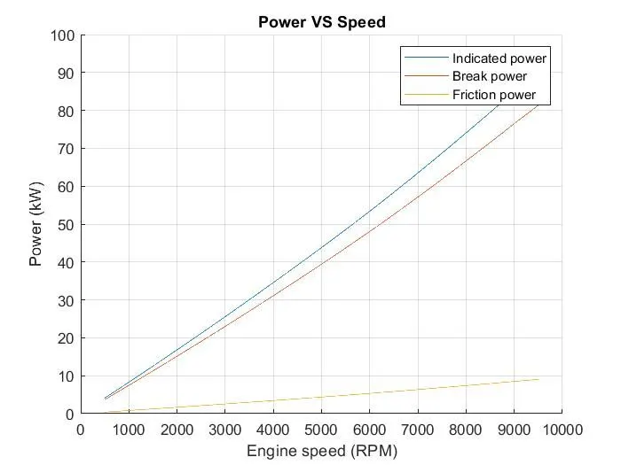
3. ENGINE POWER VS ENGINE SPEED

The x-axis represents the engine speed
The y-axis represents the engine power
The blue line represents the indicated power
The orange line represents the Brake power
The yellow line represents the friction power
Notes:
- This engine produces 81.34 kW at 9500 RPM
- The friction power loss increases with increase in engine speed

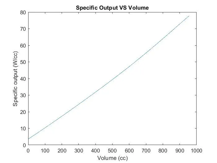
4. SPECIFIC OUTPUT VS SWEPT VOLUME

The x-axis represents the swept volume
The y-axis represents the Specific output

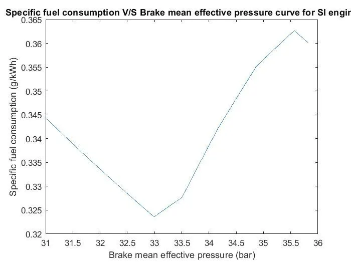
5. SFC VS BMEP

The x-axis represents the Bmep
The y-axis represents sfc

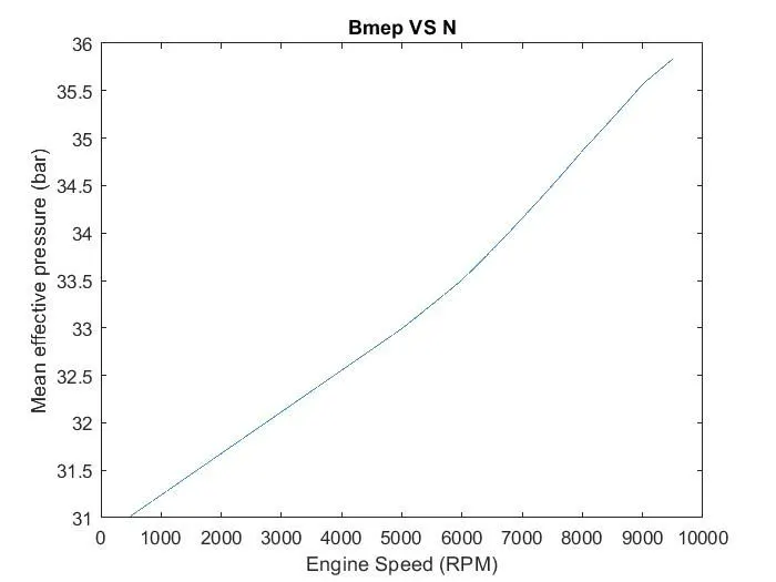
6. Bmep VS Engine Speed

The x-axis represents the engine speed
The y-axis represents the Brake mean effective pressure (Bmep)
Notes:
- Comparing plot 5 and 6, we can make the following points
  - The engine runs economically between 3000 and 4000 RPM i.e., having a specific fuel consumption between 0.3225 and 0.33 g/kWh
  - The engine at idling (500 RPM) consumes the same fuel as the engine running at 6000 RPM!
  - The engine consumes peak fuel at 8500 RPM i.e., 0.365 g/kWh