Setting up Cam Model using 3D contacts in Altair Motionview and comparing between the output of 2D and 3D contacts

https://drive.google.com/file/d/12eymt96BDEHgNr4Vt9bDlW0lAtgf4qCF/view?usp=sharing

(*The report file and the displacement result file are in different session files , in the same folder proto 10 .)

Introduction

MotionSolve contains a very sophisticated contact modeling capability that can handle complex contact scenarios between rigid bodies. Creating a contact is rather simple:

1. You can identify geometries on one body that can contact a different set of geometries on a second body.
2. You can also specify the contact material properties such as coefficient of restitution and friction.

• MotionSolve monitors the proximity of the specified geometries to each other. When any penetration between the two sets of geometries occurs, a force based on the defined contact properties is generated. This represents the contact force. Both normal as well as frictional forces are modeled.
• When the bodies separate, the force becomes zero.
• Geometries for contacts are represented through meshed surfaces. The mesh consists of interconnected triangular elements. There are several options for defining the geometry of the bodies in contact.
• There are certain criteria for the mesh geometry to be acceptable in a contact simulation:

a)The meshed surface must enclose a volume and not contain and T-connections. An enclosed volume means all elements share an edge with an adjacent element. ”T-connections” occur when more than two elements share an edge.

b) The mesh size should be relatively uniform. i.e. there should not be large variations in the length of the element edges.

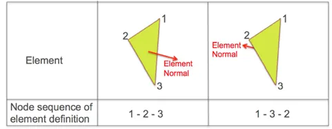
c) The element normal must point in the direction of the expected contact. The element normal is a vector which is normal to the element’s plane and along the side of the element determined by the sequence of node connection following the right hand rule as depicted in the fig below

CONTACT FORCE

• Normal Force has two components and each of the predefined method has its own way of computing these components.

F_Contact=F_spring+F_damping

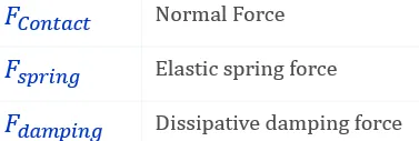
Where,The Friction Force is calculated using the Coulomb friction model.

In this case, the Coulomb friction law is used which models the friction force as a coefficient of friction multiplied by the normal force. The coefficient of friction is modeled as a function of the slip velocity.

IMPACT CONTACT MODEL

The Impact model can be thought of as a non-linear spring-damper introduced when there is penetration.

The following table lists the four parameters that define the Impact Contact Model:

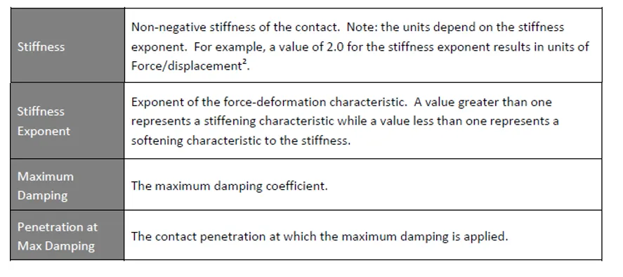
When the collision detection algorithm detects contact, the penetration depth, rate of penetration, and the above four parameters are sent to the MotionSolve IMPACT function where the normal force is calculated for each node.

Procedure

1. Import the cad model of the cam follower from the Altair's Library .

2. Import the cad model while allowing the Hypermesh to control Mesh options.(including mass and inertia )

3. Replacing the ball joint at the Follower_Roller_Joint with the Revolute joint , this will make sure the Roller doesnt moves outside the cam surface .

4. Adding the contact and making a contact between cam ( I body) and follower ( J body)

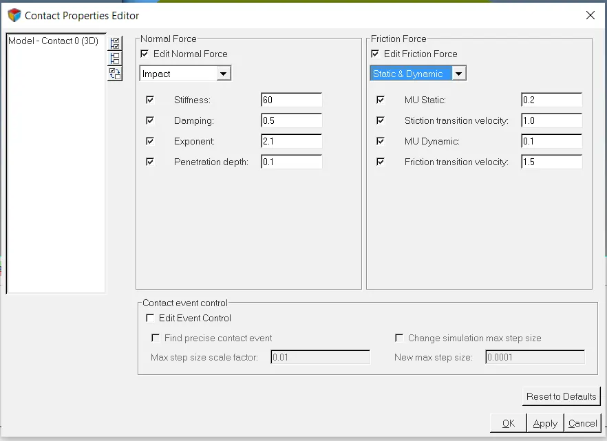
5. Go to properties tab or CONTACT PROPERTIES EDITOR .Check the 'Edit Normal Force' box and input the parameters , here we will only change the stiffness and damping value , we will gain much more information about ' why we have chosen such parametres and their values ?' in the observartion and post processing section later in the Report . Check the 'Edit friction Force ' box, enable both static and dynamic Friction. Uncheck the 'Edit Event Control' . Before completing this step , it is necessary to enable the 'IMPACT MODEL' .

6. Now input a motion at the 'CamPivot_Joint' ,under properties section give the input as an expression 'TIME/2' .

7. Make sure the Gravity is in the negative Y direction and the units of lenght is in Miliimeter .

8. Now, click on the RUN button and give the simulation time = 20 seconds .

9. Go to simulation settings ,under the Transient Tab , decrease the maximium step size to 0.001 . Change the DAE index to 1 .

10. Now run the simulation , for post processing results go to the Analysis > View Report section to see the post processing .

OBSERVATIONS AND ANALYSIS OF THE REPORT

• The two main parameters that are used in contact properties are stiffness and damping .

Stiffness :

1.

The stiffness, k, of a body is a measure of the resistance offered by an elastic body to deformation. For an elastic body with a single DOF (for example, stretching or compression of a rod), the stiffness is defined as

where,

F is the force on the body

is the displacement produced by the force along the same degree of freedom (for instance, the change in length of a stretched spring)

2.

The Elastic Modulus of a material is not the same as the stiffness of a component made from that material. Elastic modulus is a property of the constituent material; stiffness is a property of a structure or component of a structure, and hence it is dependent upon various physical dimensions that describe that component. That is, the modulus is an intensive property of the material; stiffness, on the other hand, is an extensive property of the solid body that is dependent on the material and its shape and boundary conditions. For example, for an element in tension or compression, the axial stiffness is

where

E is the (tensile) elastic modulus (or Youngs Modulus),

A is the cross sectional area ,

L is the length of the element.

3. The stiffness of a structure is of principal importance in many engineering applications, so the modulus of elasticity is often one of the primary properties considered when selecting a material. A high modulus of elasticity is sought when deflection is undesirable, while a low modulus of elasticity is required when flexibility is needed.

Hence , on the basis of the above 3 points , i have chosen the stiffness as 60 N/m ( normally most of the alloys and metals come between 30-400) , the more the youngs modulus , the more the stiffness , as the area and length remain constant .

Damping :

1. It is an influence within or upon an oscillatory system that has the effect of reducing, restricting or preventing its oscillations. In physical systems, damping is produced by processes that dissipate the energy stored in the oscillation. Examples include viscous drag in mechanical systems, resistance in electronic oscillators, and absorption and scattering of light in optical oscillators.

2. The damping ratio is a dimensionless measure describing how oscillations in a system decay after a disturbance. Many systems exhibit oscillatory behavior when they are disturbed from their position of static equillibrium. A mass suspended from a spring, for example, might, if pulled and released, bounce up and down. On each bounce, the system tends to return to its equilibrium position, but overshoots it. Sometimes losses (e.g. frictional ) damp the system and can cause the oscillations to gradually decay in amplitude towards zero or attenuate . The damping ratio is a measure describing how rapidly the oscillations decay from one bounce to the next.

3. The damping ratio is a system parameter, denoted by ζ (zeta), that can vary from undamped (ζ = 0), underdamped (ζ < 1) through critically damped (ζ = 1) to overdamped (ζ > 1).

4. Depending on the amount of damping present, a system exhibits different oscillatory behaviors.

• Where the spring–mass system is completely lossless, the mass would oscillate indefinitely, with each bounce of equal height to the last. This hypothetical case is called undamped.
• If the system contained high losses, for example if the spring–mass experiment were conducted in a viscous fluid, the mass could slowly return to its rest position without ever overshooting. This case is called overdamped.
• Commonly, the mass tends to overshoot its starting position, and then return, overshooting again. With each overshoot, some energy in the system is dissipated, and the oscillations die towards zero. This case is called underdamped.
• Between the overdamped and underdamped cases, there exists a certain level of damping at which the system will just fail to overshoot and will not make a single oscillation. This case is called critical damping. The key difference between critical damping and overdamping is that, in critical damping, the system returns to equilibrium in the minimum amount of time.

Hence , on the basis of the above 4 points , i chose the damping ratio = 0.5 which is underdamped .

• Friction

I have chosen both the static and dynamic friction for the simulation beacause in real life also an object moves only after overcoming static friction and then dynamic friction ( friction for movement ) comes into play . I have used the default values for the friction properties .

• DAE index

Setting DAE index to 1 will ensure the displacement, velocity, and acceleration of the constraints in the model are consistent. We could have also used DAE=3 .

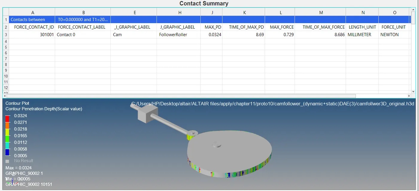
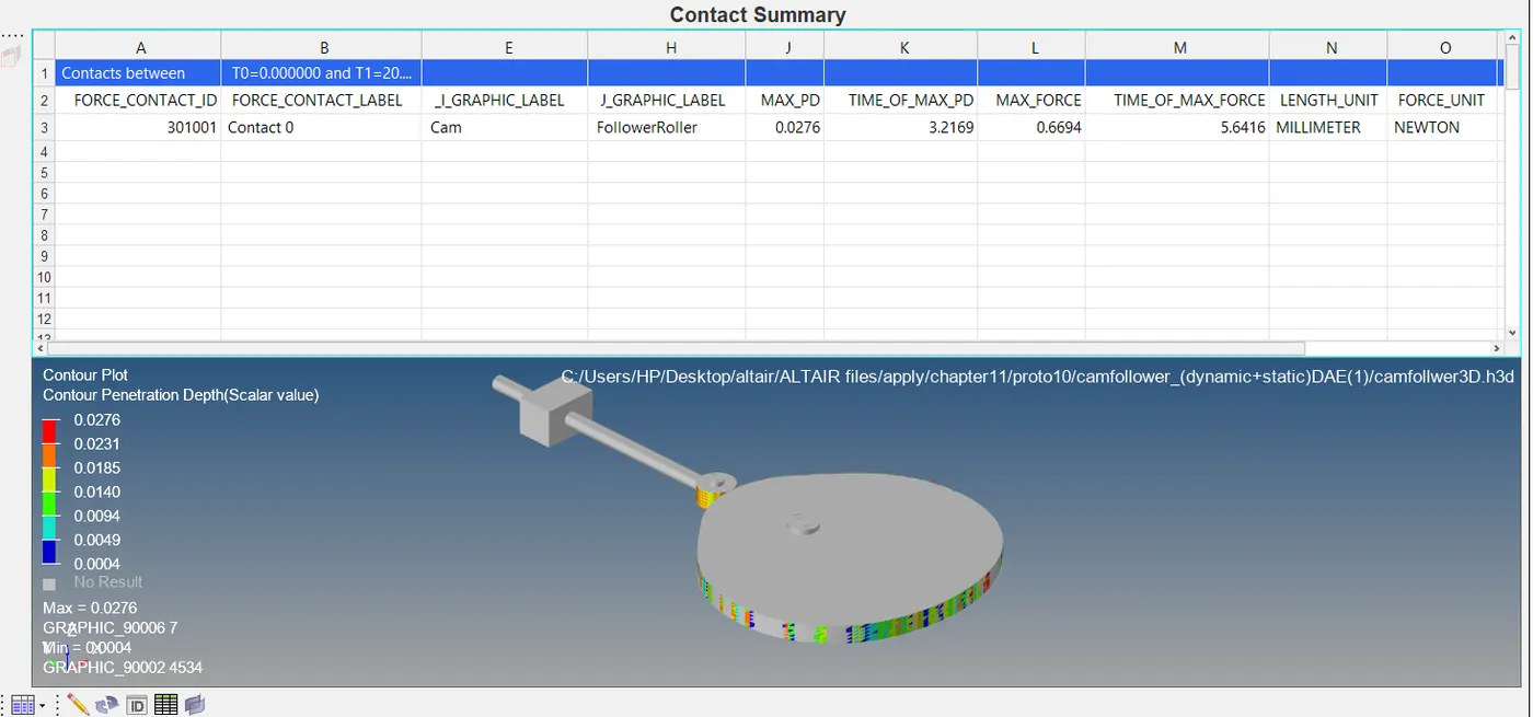
Both the DAE values that decide the simulation result , are correct , now think that if we would have made cam and follower mechanism in real , we would have seen the follower roller doing unnecessary bounce ( that relates to DAE=3 ; which is quite possible ). Now , also to improve the motion of follower roller , if we would have used spring damper system in cam and follower , we could have gotten much better mechanism with increased efficiency ( that relates to DAE=1 , which makes sure the consistency of the kinematic poperties ).I have compared the effect of DAE on the simulation .Clearly , Simulation which had DAE as 3 had higher penetration depth of 8.69 and also the follower roller was hitting the cam surface with a max force of 0.729 N, we can also see some jerky motion of follower roller in the animation file .

But with DAE of 1 , the force which was generated with the collision of follower_roller and cam was much lower i.e. 0.6694 N with penetration depth of 0.0276 quite lower than the previous case .

COMPARING CVCV JOINT AND 3D JOINT CAM-FOLLOWER DISPLACEMENT

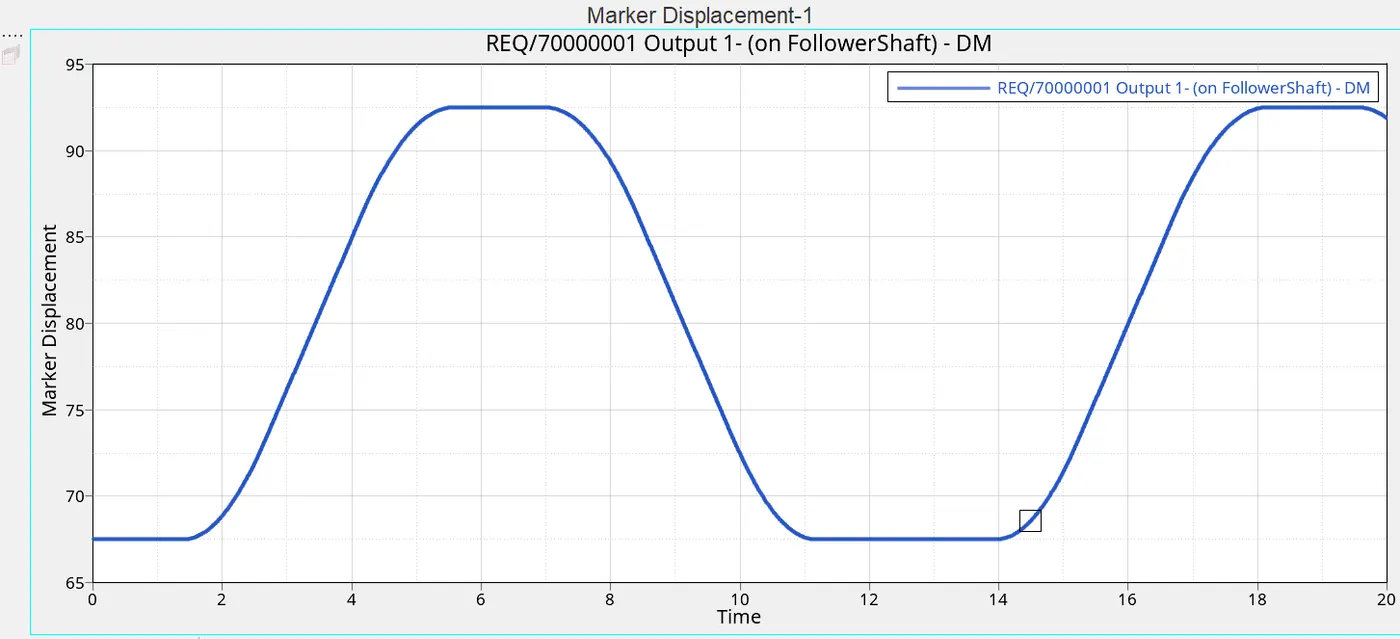
• The graphs shown below are the graphs between the displacement of follower_CM wrt the cam pivot point . The graph just below has a very smooth cam profile beacause the joint used in this case was CVCV because it provides a specific set points or a curve on which the follower_roller can travel . it restricts the movement of the roller outside that curve , this is why the roller never loses contacts with the cam .

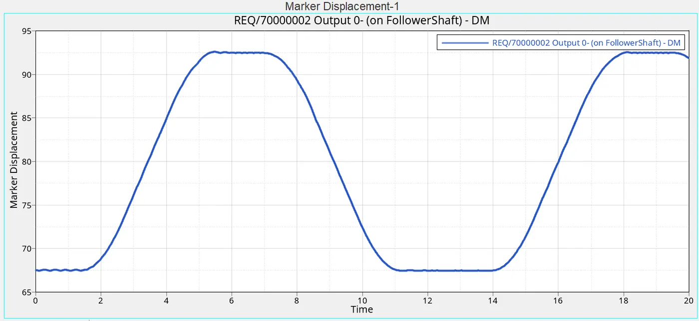
Now , in the case of 3D joint , we can see here the cam profile is not smooth . It is because the roller does not have its DOF restrained to a specific curve path , rather it is allowed to make movements by the motion on the cam , and the time_stamps where we are observing rough cuvrves is the time where the roller loses contacts with the cam surface due to the cam motion , its geometry and also some material properties like young modulus and geometrical properties like stiffness.

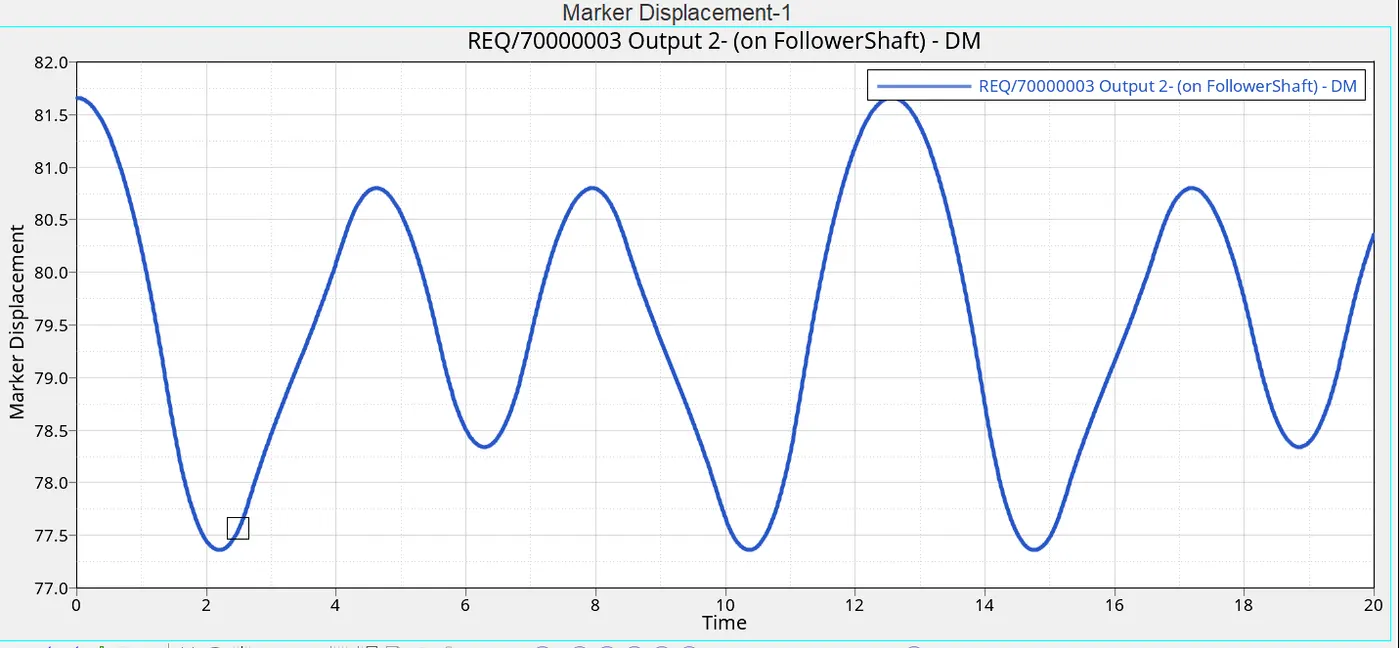
• Now this is the graph between the displacement of the follower_shaft CM vs cam_CM . The graph below shows the relative displacement between the Follower_shaft_CM AND the cam_CM , the curve again is very smooth due to the continuous contact between the surfaces of the roller and the cam (which is due to the CVCV joint )

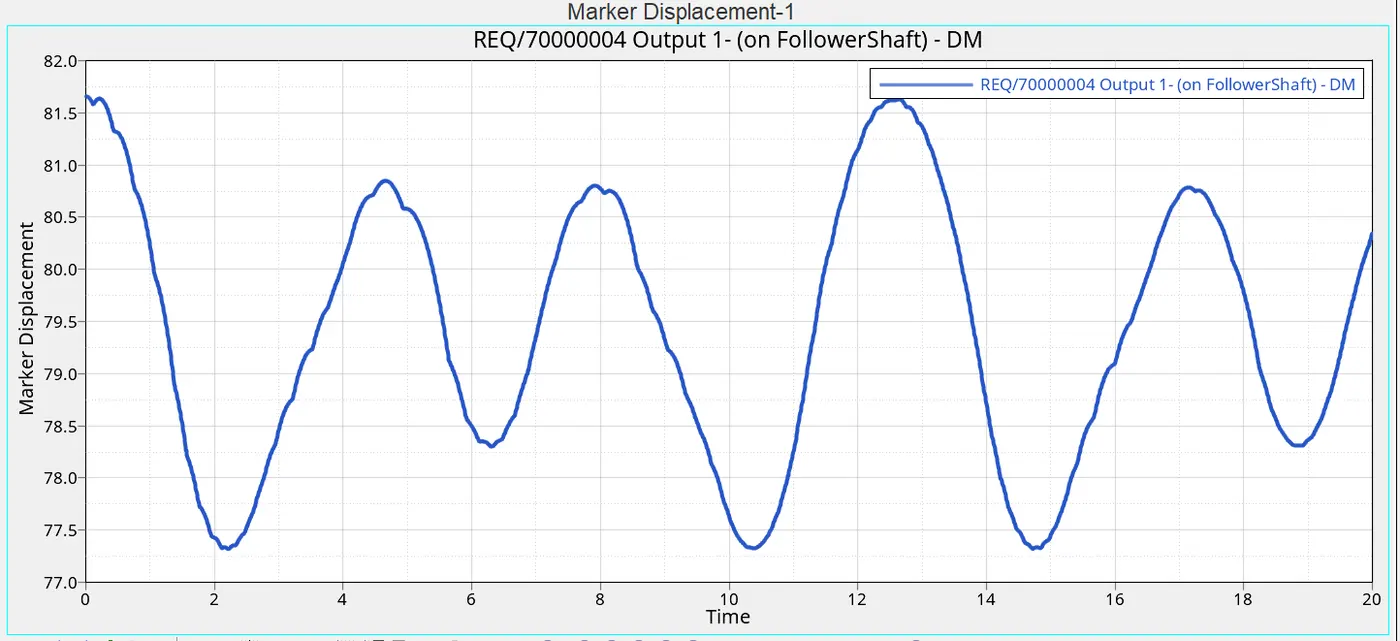
Now, in the case of Cam follower mechanism where we have used the 3D joint , we can see that the curve is not smooth , again this is due to the roller which looses its contact from the cam surface. The 3d joint is not able to properly constrain the Roller to the desired path for maximum efficiency .

Solution

• Choose best suited material for the cam_follower mechainism .
• Choose on the basis of Youngs Modulus , Stiffness .
• Use proper damping methods for the smooth motion of the follower and roller .
• Controlled lubrication to vary the friction on the contact surfaces .
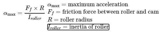
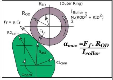
• Now , a very important thing , the roller never moves in a constant velocity or torque , it decelerates and accelerates according to the Cam Radius But in this simulation , the motion was constant ( quite false according to the real world working). Why ?

The cam-follower's outer-ring does not rotate at constant angular velocity.

Nominally, the outer-ring's of the roller :

MINIMUM ANGULAR VELOCITY is when it is in contact with the cam's Base circle ,

MAXIMUM ANGULAR VELOCITY is when it is in contact with the cam's maximum radius .

The cam-follower must accelerate and decelerate as the radius of the cam changes.However, the maximum possible angular acceleration of the cam-follower is a function of its friction, radius, and inertia. The friction-force is not constant because the contact-force is not constant, and lubrication is not steady.