Plotting the Bump Oscillation profile of various load conditions by determining the natural frequencies & making the front -rear frequencies in phase to achieve Flat ride

https://drive.google.com/file/d/15WymqKfXLtfjrMiTEQW_vIIQhwjuyMKU/view?usp=sharing

Aim

Plotting the Bump Oscillation profile of various load conditions by determining the natural frequencies & making the front -rear frequencies in phase to achieve Flat ride

Software Used

Octave , Excel

Theory

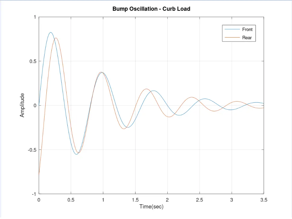
• In the graph of amplitude vs time , we will only consider first and second period as dominant because the damper helps in dying down the oscillations .
• The out of phase motion is caused because the rear hits the bump a little later than the front due to wheelbase seperation .
• If the frequencies ( front and rear ) are same , the front and rear suspension are out of phase and this causes pitching .
• For a flat ride ,the rear frequency needs to be higher than the front .
• Using a rear frequency of 1.2X the front frequency is typical .

PART 1

FLOW OF CALCULATION

• Now , we will first calculate the corner masses .
• Now , we will assume the spring rate and use it to find the wheel rate .

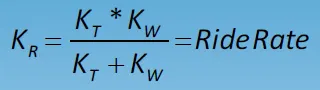
• We will calculate the ride rate using the spring and wheel rate .

• We will calculate the sprung frequency of front and rear suspensions using ride rate , corner mass , we will multiply the numerator by 1000 to convert the rates from mm to m . Same , applies to unsprung frequency , in which we will use tire rate & wheel rate and all things are same. We will change the front spring rates to get the target front sprung frequency of 1.15 hz .

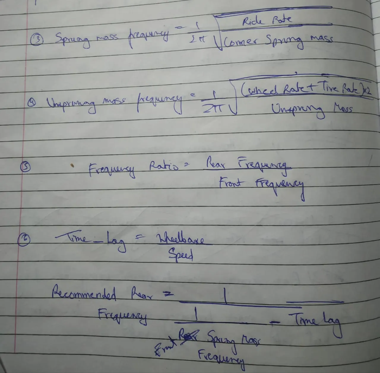
• Now , we will calculate the rear/front frequency ratio .
• Then , we will calculate the recommended rear frequency using the time lag formula , front sprung mass frequency , in excel we will multiply the wheelbase /speed from (1/0.44704) to convert mph to m/sec.
• Then we will calculate the frequency ratio .

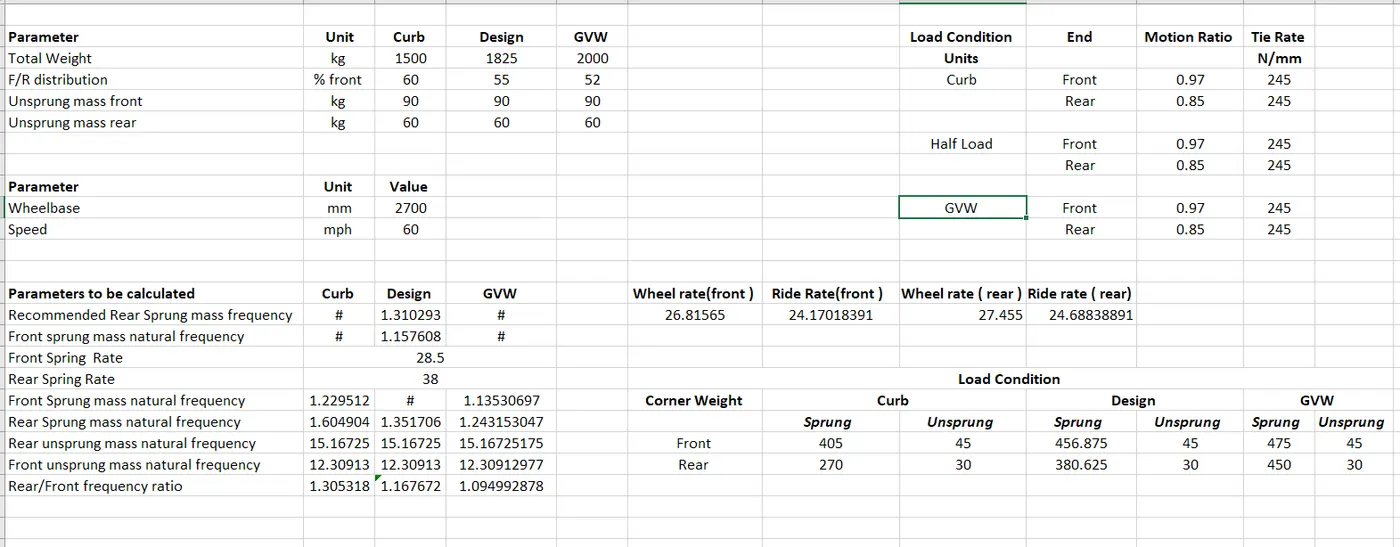
Result

Part 2

• Curb Load Bump Oscillation profile

#curb load condition 
Ws_front = 405 #kg/corner 
Ws_rear = 270 ; #kg/corner 

Ride_rate_F = 23.90085061 ; #N/mm
Ride_rate_R = 36.11054248 ; #N/mm

Timelag_wb = 0.1006621331;

freq_front=sqrt(Ride_rate_F*1000/Ws_front)/(2*pi); #hz
freq_rear=sqrt(Ride_rate_R*1000/Ws_rear)/(2*pi); #hz 

time=[0:0.01:3.5]

i=1;
for t=0:0.01:3.5 ;
  front_amp(i) = exp(-t)*sin(2*pi*freq_front*t);
  rear_amp(i) = exp(-t)*sin(2*pi*freq_rear*(t-Timelag_wb));
  i+=1;
end

figure ();
plot(time,front_amp);
hold 
plot(time,rear_amp);
grid on;
hold off;

title('Bump Oscillation - Curb Load');
xlabel('Time(sec)');
ylabel('Amplitude');
legend('Front','Rear');

Output

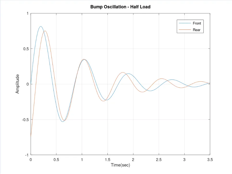
• Half Load Bump Oscillation

#Half load condition 
Ws_front = 456.875 #kg/corner 
Ws_rear = 380.625 ; #kg/corner 

Ride_rate_F = 24.7 ; #N/mm
Ride_rate_R = 26 ; #N/mm

Timelag_wb = 0.1006621331;

freq_front=sqrt(Ride_rate_F*1000/Ws_front)/(2*pi); #hz
freq_rear=sqrt(Ride_rate_R*1000/Ws_rear)/(2*pi); #hz 

time=[0:0.01:3.5]

i=1;
for t=0:0.01:3.5 ;
  front_amp(i) = exp(-t)*sin(2*pi*freq_front*t);
  rear_amp(i) = exp(-t)*sin(2*pi*freq_rear*(t-Timelag_wb));
  i+=1;
end

figure ();
plot(time,front_amp);
hold 
plot(time,rear_amp);
grid on;
hold off;

title('Bump Oscillation - Half Load');
xlabel('Time(sec)');
ylabel('Amplitude');
legend('Front','Rear');

Output

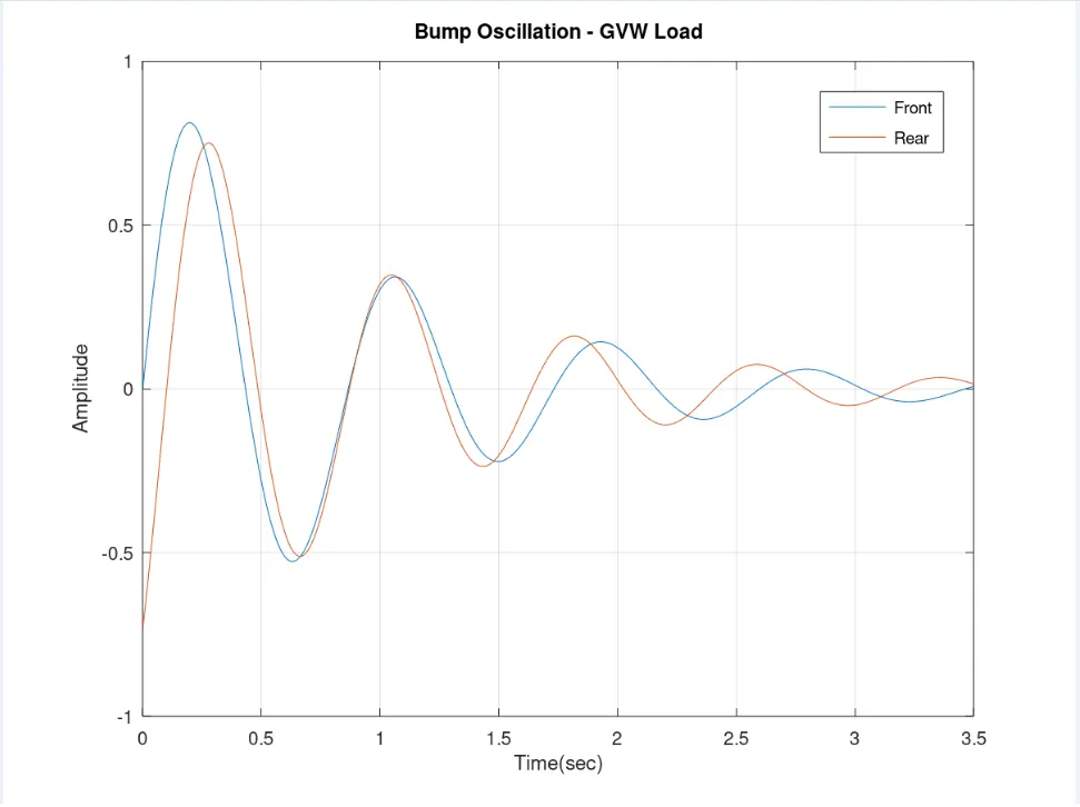
GVW Bump Oscillation Profile

#GVW load condition 
Ws_front = 475 #kg/corner 
Ws_rear = 450 ; #kg/corner 

Ride_rate_F = 25 ; #N/mm
Ride_rate_R = 30 ; #N/mm

Timelag_wb = 0.1006621331;

freq_front=sqrt(Ride_rate_F*1000/Ws_front)/(2*pi); #hz
freq_rear=sqrt(Ride_rate_R*1000/Ws_rear)/(2*pi); #hz 

time = [0:0.01:3.5];


i=1 ;
for t=0:0.01:3.5 ;
  front_amp(i) = exp(-t)*sin(2*pi*freq_front*t);
  rear_amp(i) = exp(-t)*sin(2*pi*freq_rear*(t-Timelag_wb));
  i+=1;
end

figure ();
plot(time,front_amp);
hold 
plot(time,rear_amp);
grid on;
hold off;

title('Bump Oscillation - GVW Load');
xlabel('Time(sec)');
ylabel('Amplitude');
legend('Front','Rear');

Output

Result

The frequencies of the front and rear were made in phase ( in all three load conditions namely : Curb , Half , GVW ) to achieve the main goal of acheiving a flat ride . The front and rear frequency multiplying factor for different load conditions vary from ( 1.09-1.30) .