Setting up Cam Model using 2D contacts in Altair Motionview

https://drive.google.com/file/d/1sH3NdGG1RWKqikIlo9Whsyv5PcDpG5y1/view?usp=sharing

INTRODUCTION

The kinematic pair is very important aspect to understand in theory of Machines.
The classification of kinematics pair, the most important one is based on the point of contact. On that basis kinematics pair are of two types. These are Lower pair and higher pair

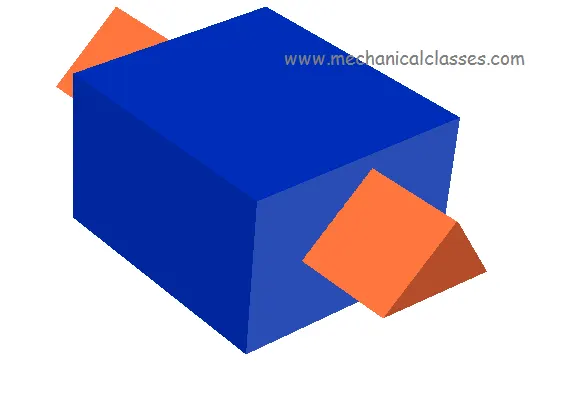
• Lower pair : A lower pair is an ideal joint that constrains contact between a surface in the moving body to a corresponding surface in the fixed body. A lower pair is one in which there occurs a surface or area contact between two members.For example : Prismatic joint . Prismatic joint is a lower pair which has one directional translatory motion and has degree of freedom = 1. This means Prismatic joint has constraint in 5 directions.

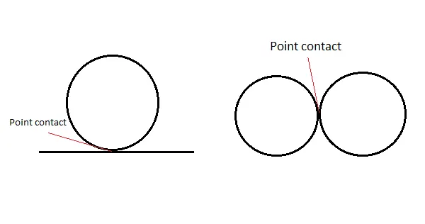
• Higher pair : Generally, a higher pair is a constraint that requires a curve or surface in the moving body to maintain contact with a curve or surface in the fixed body. For example, the contact between a cam and its follower is a higher pair called a cam joint. It has a point or line contact.

Cam Follower Mechanism

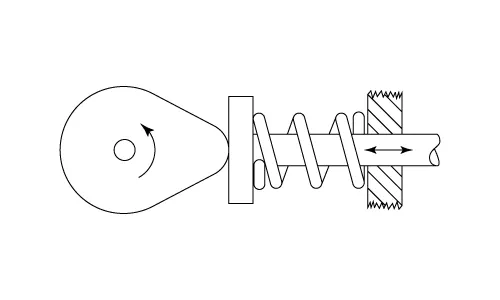
A cam is a rotating or sliding piece in a mechanical linkage used especially in transforming rotary motion into linear motion. It is often a part of a rotating wheel (e.g. an eccentric wheel) or shaft (e.g. a cylinder with an irregular shape) that strikes a lever at one or more points on its circular path. The cam can be a simple tooth, as is used to deliver pulses of power to a steam hammer. A cam timer is similar, and were widely used for electric machine control (an electromechanical timer in a washing machine being a common example) before the advent of inexpensive electronics.

In general the motion of the follower is only determined positively by the cam during a part of each stroke whilst during the remainder of the stroke contact between the cam and the follower has to be maintained by an external force, often supplied by a spring. In this connection it should be noticed that the cam does not, as would at first appear likely, determine the motion of the follower during the whole of the its out-stroke. Actually, owing to the inertia of the follower, it is only during the first part of the out-stroke and the latter part of the return that the motion of the follower is positively controlled by the cam.

Types of Cam :

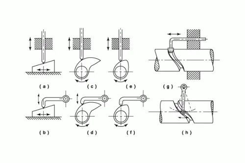
Cams are classified according to the direction of displacement of the follower with respect to the axis or oscillation of the cam. The two most important types are :

• Disc or Radial Cams In these the working surface of the cam is shaped that the reciprocation or oscillation of the follower is in a plane at right angles to the axis of the cam. ( see examples c; d; e; f above )
• Cylindrical Cams These are often used in machine- tools and the cam imparts an oscillation or reciprocation to the follower in a plane parallel to the axis of the cam. ( see examples g and h above)

Types of Follower

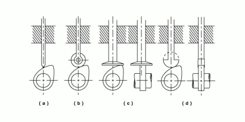
1. Knife edged. These are not often used due to the rapid rate of wear of the knife edge.
2. Roller Follower. The roller follower has the advantage that the sliding motion between cam and follower is largely replaced by a rolling motion. Note that sliding is not entirely eliminated since the inertia of the roller prevents it from responding instantaneously to the change of angular velocity required by the varying peripheral speed of the cam.
3. Flat or Mushroom Follower.The relative motion is one of sliding but it may be possible to reduce this by off setting the axis of the follower as shown in the diagram. This results in the the follower revolving under the influence of the cam.
4. Flat faced Follower. These are really an example of the mushroom follower and are used where space is limited. The most obvious example being automobile engines.

Procedure

• We will open the cam_follower model from the Altair library .
• First , deactivate the previous cam model in the body section along with the graphic .
• Now, first we will design a elliptical cam using solidworks , with the dimensions ( major axis : 25 mm , minor axis : 15 mm )

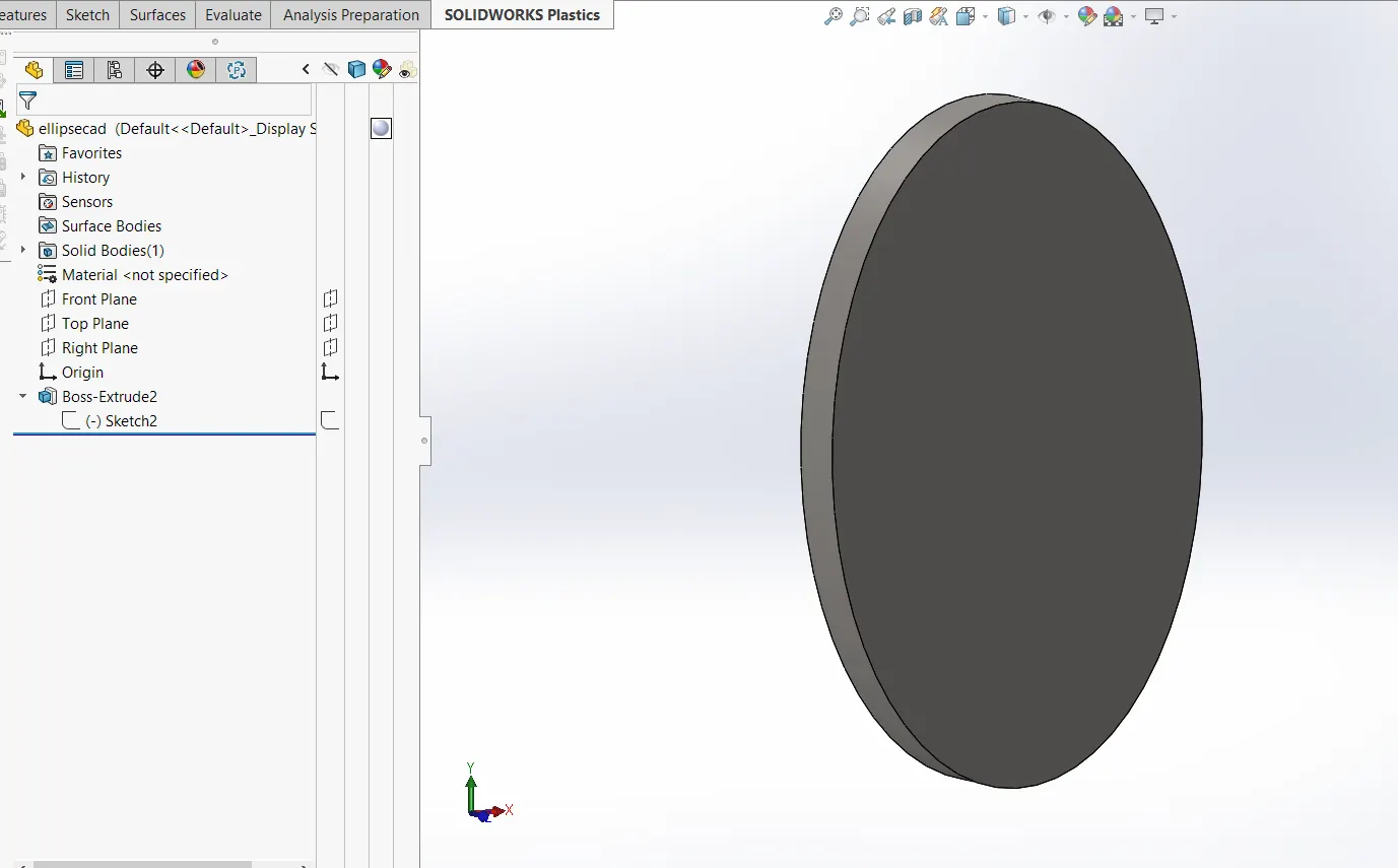
• Now , import the cad model with mass and inertia . Let the hypermesh control the mesh of the imported cad model .
• Now , before importing check whether the gravity is in -ve direction and the length unit is in millimeter .
• After importing the cad model , delete the previous cam graphic and body .
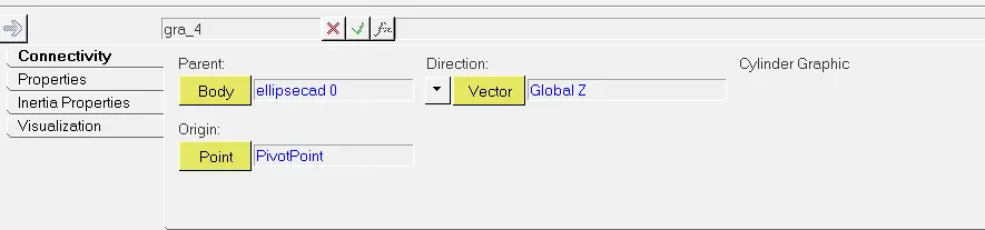
• Now , add cam_pivot_graphic at the new cam ( ellipse_0 )

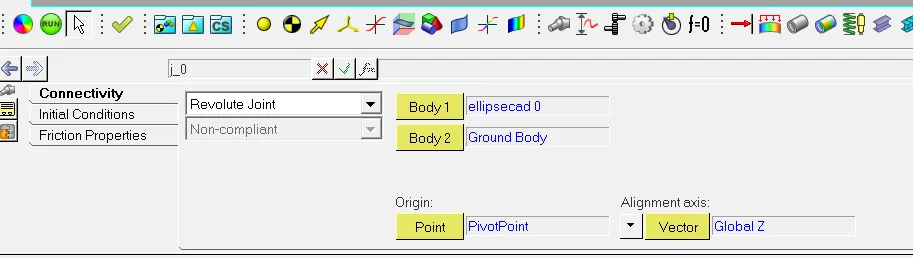
• Now , connect cam_pivot joint between cam and the ground .

• Update the cam marker , associate it with cam body and attach it to the pivot_point .
• Create a cam motion at the campivot with expression (5*TIME) .
• Now add two curves using math function one for roller and one for cam .

Curve for the cam generated using math function for x coordinates : { 15*sin(2*PI*(0:1:0.01)) }

y coordiantes : {25*cos(2*PI*(0:1:0.01)) }

z coordinates : { 0*sin(2*PI*(0:1:0.01)) }

Curve for the follower_roller using math function for x coordinates : { 5*sin(2*PI*(0:1:0.01)) }

y coordinates : {5*cos(2*PI*(0:1:0.01)) }

z coordinates : { 0.0*(0:1:0.01) }

We will choose 3D cartisian system along with the closed curve feature .

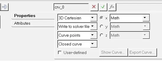
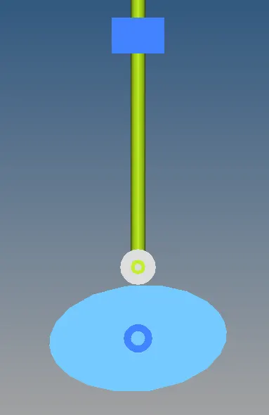
Now ,after the curve generation the cam and roller will look like this

• Now , we will add one advanced joint . We will choose CVCV joint from the drop down list . Then , we will specify marker for cam and roller . We will add curves associated with the two bodies and finally the bodies will be generated in the advanced joint coloumns .

• Now , we will add output to study the torqe about the z axis , for this we will use CVCV output function which comes under the force section . But before that let us know the details of this function .

Format : CVCV (id, jflag, comp, rm)

Arguments id : An integer specifying the identification member of the bushing.

jflag : An integer flag specifying the bushing connectivity marker at which the
forces and torques are computed.

0 = forces and moments at the I marker
1 = forces and moment at the J marker

comp : An integer value that specifies the component of the bushing force to be
returned.

1 = Magnitude of the force
2 = x component of the force
3 = y component of the force
4 = z component of the force
5 = Magnitude of the torque
6 = x component of the torque
7 = y component of the torque
8 = z component of the torque

rm :The coordinate system in which the results are expressed. To return the
results in the global coordinate system, set rm = 0.

Hence the CVCV output function was CVCV({aj0.idstr∈g},0,8,0)">CVCV({aj0.idstr∈g},0,8,0)CVCV({aj0.idstr∈g},0,8,0)

• Now , we will add some displacements graph to study the cam profile of the elliptical cam between the CM of the follower shaft and CM /cam_pivot point .
• We will click on the run button , we will change the DAE index value to 1 ( Because it will control the velocity , acceleration to make it more smooth or consistent ).
• We are ready to run the simulation, enter the simulation duration and run the simulation.

Studying the ouputs

• First , we will look at the displacement output or the cam profile

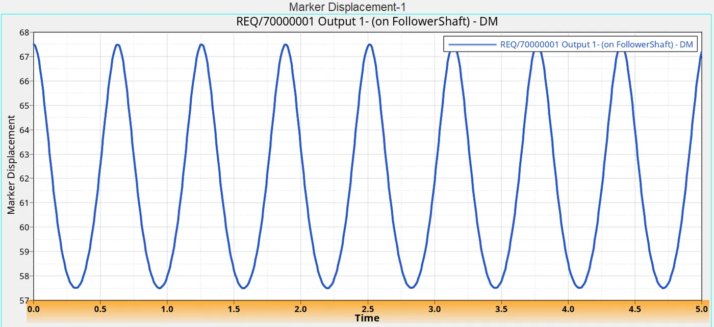
Clearly , when the ellipse cam rotates for about 90 degrees about the Z axis , at that time , the follower_CM reaches to the lowest y (displacment ) of the graph . When the ellipse covers another 90 degrees , the Follower_CM reaches to its original position or the highest y value of the displacement graph .

• Now , we will look at the torque generated about the Z axis .

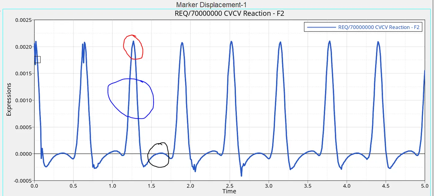
This graph was generated using the I marker in CVCV function . The red zone is where the elliptical cam reaches its original position ( when the cam reaches its full height ) ,the torque is maximum at this point because the torque depends upon distance also along with the force ( contact force ) , at this point due to increase in the distance the torque increases . In the blue zone , we can see the torque decrease ,we can see a sharp decline because we know the cam's angular acceleration always varies due to its varying radii , the formula that explains this is :

The surface where the radii becomes maximum , the angular acceleration increases , angular velocity increases , thus torque increases ; same is possible for the minimum radii and vice versa . But in the graph we can see torque becoming negative , it could happen when there is slight lose of contact or the cam reverses direction for a very small amount of time due to some causes like friction , surface of the cam or machine error . Though the torque generated is very small . In the black zone we can see that the torque reaches 0 and remains close to 0 for small time which is also due to the radii of the elliptical cam which does not changes much due to a less radial change of the surface as we can see in the figure .