Rayleigh Taylor Instability Challenge
Aim:
1.Explian CFD models that have been based on the mathematical analysis of Rayleigh Taylor waves.
2.Perform the Rayleigh Taylor instability simulation for 2 different mesh sizes with the base mesh being 0.5 mm. Compare the results by showing the animations and Observe the differences in the animation
3.explain the effect of mesh size on simulation. Also, explain why a steady-state approach might not be suitable for these types of simulation.
4.Define the Atwood Number. Find out the Atwood number for both the cases and explain how the variation in Atwood number in the above two cases affects the behavior of the instability.
Rayleigh–Taylor instability:
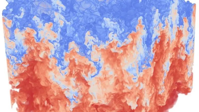
1. Rayleigh–Taylor instability given after lord rayleigh and G I Taylor is an instability of an interfernce between two fluids of different densities.which occurs when the lighter fluid is pushing the heavier fluid.
2.Examples include the behavior of water suspended above oil in the earths gravity,mushroom clouds like those from volcanic eruptions and atmospheric nuclear explosions.
3.supernova explosions in which expanding core gas is accelerated into denser shell gas, instabilities in plasma fusion reactors and inertial confinement fusion.
4.Water suspended atop oil is an everyday example of Rayleigh–Taylor instability.
5.it is modled by two completely plane-parallel layers of immiscible fluid, the more dense on top of the less dense one and both subject to the Earth's gravity.
6. Fluids are accelerated with the less dense fluid accelerating into the more dense fluid. This occurs deep underwater on the surface of an expanding bubble and in a nuclear explosion
7.As the RT instability develops, the initial perturbations progress from a linear growth phase into a non-linear growth phase, eventually developing "plumes" flowing upwards and "spikes" falling downwards.
8.In the linear phase, the fluid movement can be closely approximated by linear equations, and the amplitude of perturbations is growing exponentially with time.
9.In the non-linear phase, perturbation amplitude is too large for a linear approximation, and non-linear equations are required to describe fluid motions.
10.In general, the density disparity between the fluids determines the structure of the subsequent non-linear RT instability flows (assuming other variables such as surface tension and viscosity are negligible here).
Practical cfd models based on rayleigh taylor instability:
1. Richtmyer-Meshkov instability
1. The Richtmyer–Meshkov instability occurs when two fluids of different density are impulsively accelerated. Normally this is by the passage of a shockwave
2.The development of the instability begins with small amplitude perturbations which initially grow linearly with time.
3.This is followed by a nonlinear regime with bubbles appearing in the case of a light fluid penetrating a heavy fluid, and with spikes appearing in the case of a heavy fluid penetrating a light fluid.
4.A chaotic regime eventually is reached and the two fluids mix. This instability can be considered the impulsive-acceleration limit of the rayleigh taylor instability
5.This review focuses on the basic physical processes underlying the onset and development of the Richtmyer-Meshkov instability in simple geometries.
6.Supersonic combustion in a scramjet may benefit from RMI as the fuel-oxidants interface is enhanced by the breakup of the fuel into finer droplets. Also in studies of(DDT) processes show that RMI-induced flame acceleration can result in detonation.
2.Kelvin–Helmholtz instability
1.The Kelvin–Helmholtz instability typically occurs when there is velocity shear in a single continous fluid
2. additionally where there is a velocity difference across the interface between two fluids.
3. common example is seen with wind blowing over water, the instability constant is able to manifest itself through waves on a water surface.
4.The Kelvin-Helmholtz instability is not only restricted to a water surface as clouds, but is evident through other natural phenomena as the ocean, Saturn's bands, Jupiters red spot, and the sun's corona
3.Plateau–Rayleigh instability
1.The Plateau–Rayleigh instability, often just called the Rayleigh instability, explains why and how a falling stream of fluid breaks up into smaller packets with the same volume but less surface area.
2.It is related to the Rayleigh taylors instability and is part of a greater branch of fluid dynamics concerned with fluid thread brakeup.
3.This fluid instability is exploited in the design of a particular type of ink jet technology whereby a jet of liquid is perturbed into a steady stream of droplets.
4.The driving force of the Plateau–Rayleigh instability is that liquids, by virtue of their surface tensions, tend to minimize their surface area. A considerable amount of work has been done recently on the final pinching profile by attacking it with self-similar solutions.
steady-state approach:
1.Steady-state flow refers to the condition where the fluid properties at a point in the system do not change over time.
2.steady state focouses on end results
2.Time dependent flow is known as unsteady (Transiant)
3. For intermixing of fluids transiant state approach is better for proper visualization and gives clear picture at intermediate stage.
4.we can record simulation for each time step in transiant state.
.
Atwood number:
The Atwood number (A) is a dimensionless number in fluid dynamics used in the study of hydrodynamic instabilities in density stratified flows.
1.In Rayleigh–Taylor instability, the penetration distance of heavy fluid bubbles into the light fluid is a function of acceleration time scale, 

where
 = density of heavier fluid
 = density of lighter fluid
Case1: ρ1=998 and ρ2=1.225 then A= 0.99754
Case2: ρ1=998 and ρ2=400 then A= 0.42775
Effect of Atwood number:
1.Atwood number close to 0 RT instability flows take the form of symmetric "fingers" of fluid
2.Atwood number close to 1 much lighter fluid "below" the heavier fluid takes the form of larger bubble-like plumes
3.Atwood number far from 1 difficult to identify whether it is bubble or spike because of variation in density is negligible.
Procedure:
Geometry:
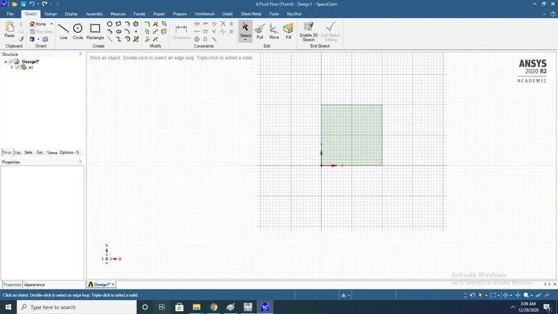
1.Draw square of dimensions (20mm*20mm) named as air less dense at bottom.
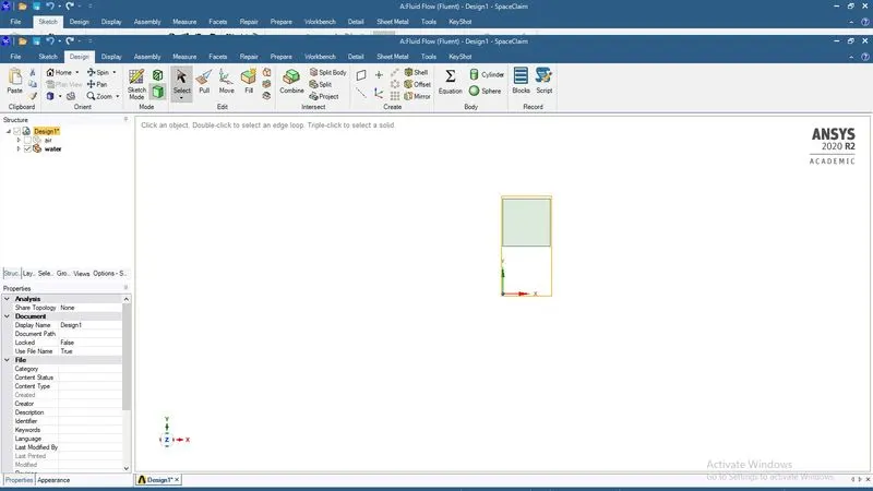
2.Draw square of dimensions (20mm*20mm) named as water more dense at top.
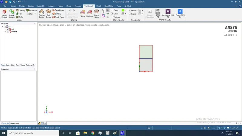
3.Next select entire drawing and enable share and click on enable so that topology is shared
Meshing:
Grid dependency test:
1.Apply simple mesh by maintaining element size=0.5 and generate
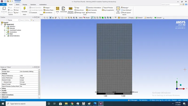
2. No of elements= 3200
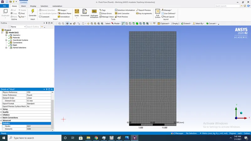
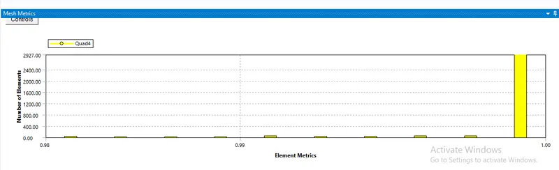
3.Element quality
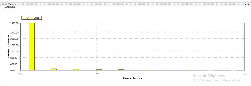
3.Aspect ratio
Grid dependency test:
1.Apply simple mesh by maintaining element size=0.2 and generate
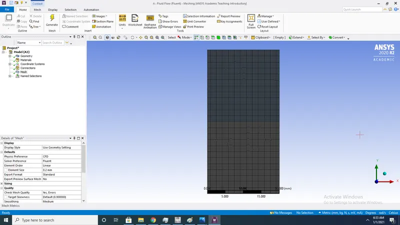
2. No of elements= 20000
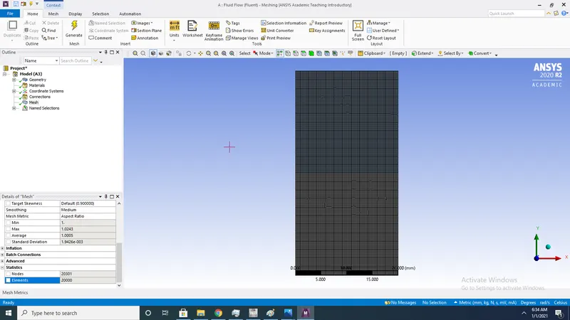
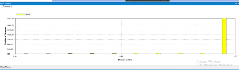
3.Element quality
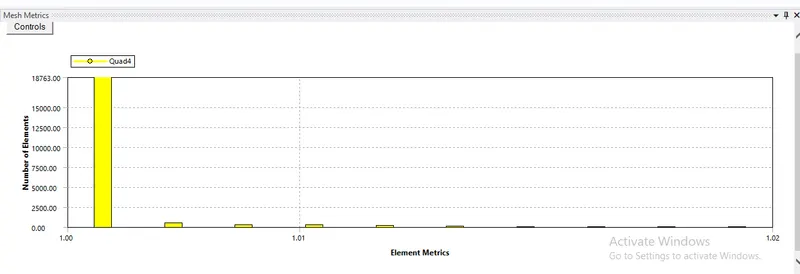
4.Aspect ratio
Setup:
1)General
Type: Pressure-based
Time: Tansiant
Velocity formulation: Absolute
2D Space : Planar
2)Models:
Viscous: Laminar
3)Materials:
case1:
Density of air =1.225(kg/m^3) Density of water= 998 (kg/m^3)
case2:
Density of water= 998 (kg/m^3) density of user defined=400 kg/m3
4)Multi phase : On
5) Enable implicit method and use primary phase as air and secondary phase as water (Case1)
6) Enable implicit method and use primary phase as air and secondary phase as user defined (Case2)
7) Next intialize hybrid solution after intialization do patch first do patch for water and volume fraction for water=1 and next patch for air and volume fraction=0
8) Next intialize hybrid solution after intialization do patch first do patch for water and volume fraction for water=1 and next patch for user defined and volume fraction=0
9) Next plot contours of phases and volume fraction of water
10)next click on auto save for time step animations
11)next run iterations for time step size=5e-3 and no of iterations=1000
Contours:
for mesh size=0.5mm
Phase countor
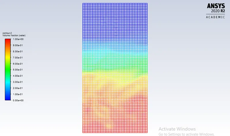
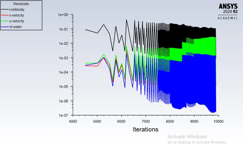
Residuls:
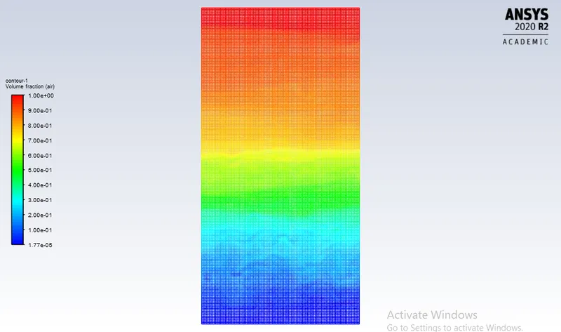
For mesh size=0.2mm
Phases contour:
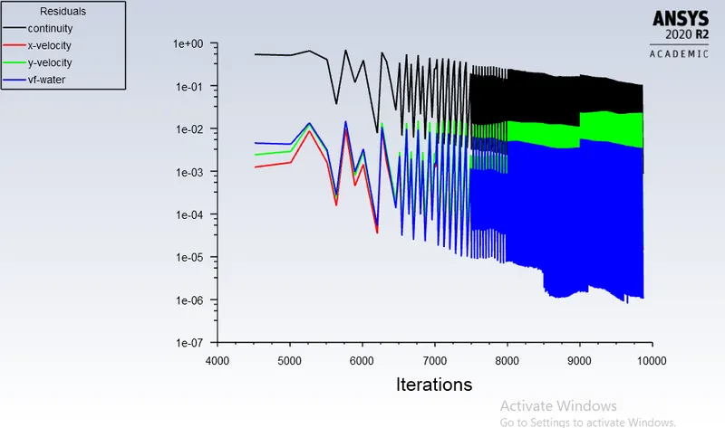
Residuals:
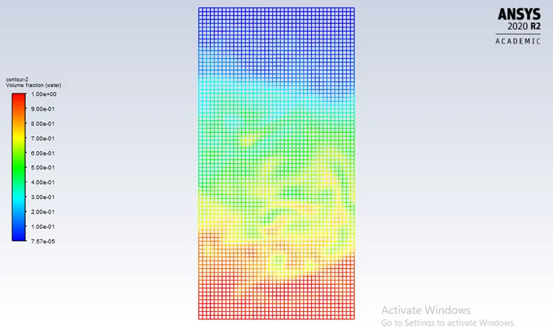
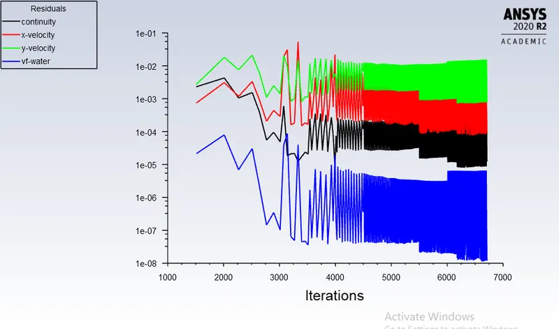
For mesh size=0.5mm (User defined material)
Phases contour:
Residuals:
Animations:
https://drive.google.com/file/d/1hBPJKxZt0Ybblkdz6p63SNEOmBGwIpth/view?usp=sharing
https://drive.google.com/file/d/1PMtANkIUBoDbdMisNKjJSZA_EQE3Rx77/view?usp=sharing
https://drive.google.com/file/d/177d5noBDHFZZdk3n70H58r54PbB0WnQj/view?usp=sharing
Observations:
1. finer mesh gives better results compared to coarse mesh size on comparing mesh size of 0.2 and 0.5 instability settle down for mesh size of o.2
2. simulation time increases for finer mesh sizes but gives better results.