Rayleigh Taylor Instability Challenge
Aim: The aim of the challenge is to perfrom Rayleigh Taylot Instability simulation for differnt mesh size and also learn the significance of Atwood number.
Objective:
1.Perform the Rayleigh Taylor instability simulation for 2 different mesh sizes with the base mesh being 0.5 mm.
2.Run one more simulation with water and user-defined material(density = 400 kg/m3, viscosity = 0.001 kg/m-s) for refined mesh.
3.Define the Atwood Number. Find out the Atwood number for both the cases and explain how the variation in Atwood number in the above two cases affects the behavior of the instability.
Rayleigh Taylor instability in our daily life:
Our everyday experience we know that atmospheric pressure cannot support even a few centimeters of water within a glass container when it is inverted. The reason for this apparent contradiction is the characteristic instability of the equilibrium configuration in which water, the denser fluid, lies above the
less dense air. Situations of unstable equilibrium are very common in mechanical systems, but in fluids instabilities manifest themselves sometimes in a spectacular way. Furthermore, the inherent physical mechanisms underlying the development of an instability are frequently not intuitive. The instability of a dense fluid above a lower density fluid in a gravitational field is known as the Rayleigh-Taylor instability in honor of Lord Rayleigh, who first described itmathematically in 1883, and Sir G. Taylor, who in 1950
demonstrated that the instability can also occur in accelerated fluids.The first experiment to validate the theory was conducted by Lewis in 1950.The Rayleigh-Taylor instability is one of the hydrodynamic instabilities that is easiest to observe. It is not only responsible for the water falling when we invert a glass but it also plays an important role in many natural processes ranging from coastal upwelling, which helps to renew the nutrients near the surface of the sea, to the ignition of a supernova at the end of the life of some stars.The RayleighTaylor instability is present in the formation of some astrophysical structures such as the supernova remnants in the Eagle and Crab nebula,in the air bubble formation in
the blood of deep sea divers, and in many industrial processes.
Geometry:
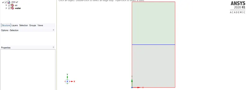
We have created the below geometry using rectangles for two fluids in consideration one above the other with dimension 20*20 mm.
Meshing:
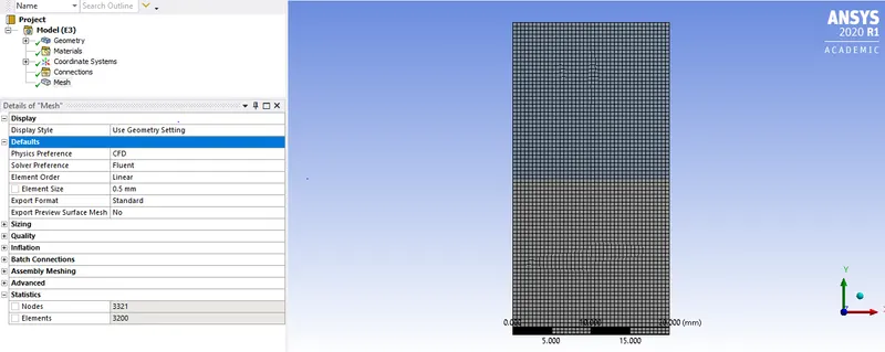
The baseline mesh is generated initially to run the setup with mesh size of 0.5 mm.
No of nodes:3321
No.of elements:3200
Solution setup:
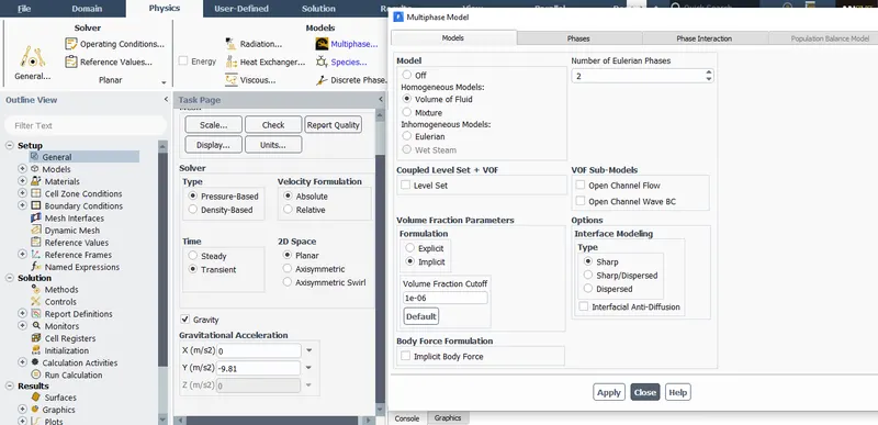
For the solution setup of the simulation solver-pressure based,velocity formulation-absolute,time-transient,2d space-planar,viscous model-laminar.
Gravitational accelaration= -ve 9.81 m/s2 in y direction.
Material:we use fluent data base and select water liquid and air as material.
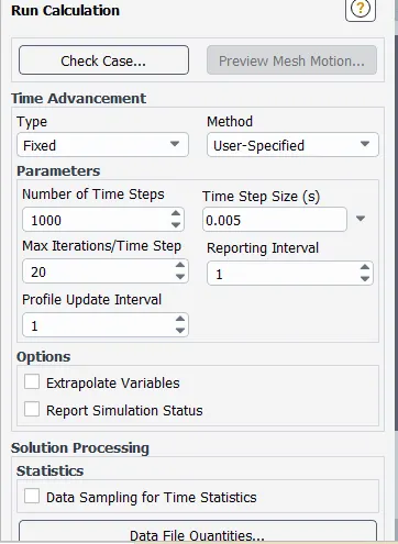
For multiphasemodeling we do the following settings as shown below for our fluids air and water.
for the part 2 we use user defined fluid instead of air.
Phase 1 is air and phase 2 is water
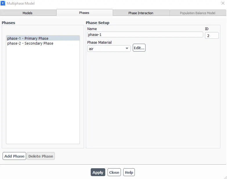
Standard initialization is done and patching is required in order to make sure that the air is in the lower side of geometry and water is in upper side of geometry to begin simulation.
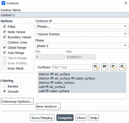
Countour of phase and volume fraction is ploteed and animation file is generated
Case 1) Baseline Mesh with mesh size 5mm
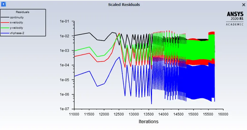
Residual plot:
Animation:
Case2: Mesh size 0.3mm
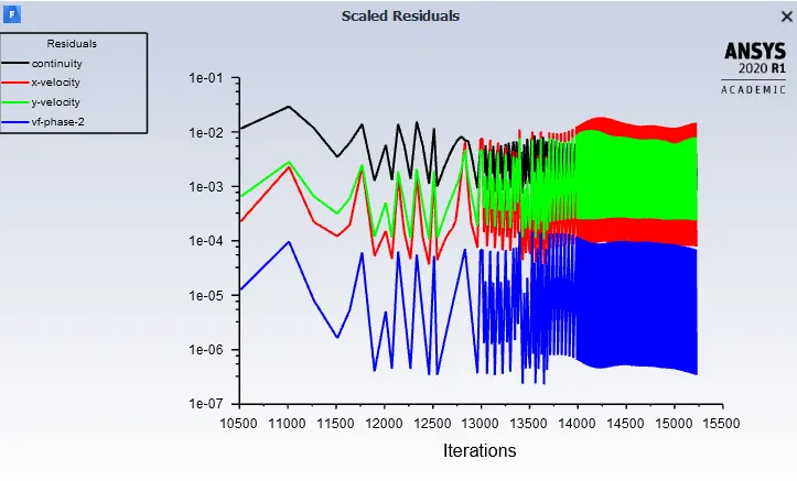
Residual plot:
Animation:
Case 3: Mesh size 0.2 mm
Residual plot:
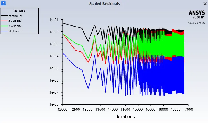
Animation:
Case 4: User defined material with density = 400 kg/m3, viscosity = 0.001 kg/m-s and mesh size of 0.5 mm
Residual plot:
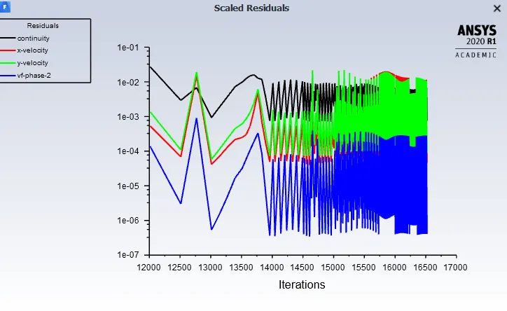
Animation:
Results:
From the observations made with varying mesh size we can say that baseline mesh of 0.5 mm gives very unrefined result that is it doesnt catch the flow very effciently as compared to more refined mesh size of 0.3 or 0.2 mm.but with increase in refinement of mesh the number of elements also increases which increases the use of computaional time and space.
why a steady-state approach might not be suitable for these types of simulation?
we have used transient approach to view the flow at every time step which is not possible with steady state approach which gives us end result.as we are supposed to observe the flow that is taking place when two fluids comes in contact and mixes together.the steady state approach is suitable only when we want to visualize the end result or equilibruim.
Atwood number:
The Atwood number (A) is a dimesnsionless number in fluid dynamics used in the study of hydrodynamic instabilities in density stratified flows. It is a dimensionless density ratio defined as

where
 = density of heavier fluid
 = density of lighter fluid
Case 1) Air: density= 1.225 kg/m3 water: density=998.2 kg/m3
therefore Atwood number A=998.2-1.225/998.2+1.225=0.9975
Case 2) user defined material: density= 400 kg/m3 water: density=998.2 kg/m3
therefore Atwood number A=998.2-400/998.2+400=0.4278
Atwood number is an important parameter in the study of Rayleigh Taylot Instability. In Rayleigh–Taylor instability, the penetration distance of heavy fluid bubbles into the light fluid is a function of acceleration time scale,  where g is the gravitational acceleration and t is the time.