Rayleigh Taylor Instability Challenge
Problem Definition
1. What are some practical CFD models that have been based on the mathematical analysis of Rayleigh Taylor waves? Explain how these mathematical models have been adapted for CFD calculations.
2. Perform the Rayleigh Taylor instability simulation for 2 different mesh sizes with the base mesh being 0.5 mm. Compare the results. Observe the differences in the animation and explain the effect of mesh size on simulation. Also, explain why a steady-state approach might not be suitable for these types of simulations.
3. One simulation with water and user-defined material(density = 400 kg/m3, viscosity = 0.001 kg/m-s) for refined mesh.
4. Define the Atwood Number. Find out the Atwood number for both the cases and explain how the variation in Atwood number in the above two cases affects the behavior of the instability.
Introduction
Rayleigh Taylor instability
The Rayleigh–Taylor instability (RTI) is the instability of an interface between two fluids of different densities which occurs when the lighter fluid is pushing the heavier fluid.
Rayleigh-Taylor instability (RTI) is the interpenetration of materials that occurs whenever a light fluid pushes on a heavy fluid. It is a dynamic process whereby the two fluids seek to reduce their combined potential energy. RTI to occur is when two layers of fluid are set on top of each other under constant gravity, with the heavy fluid with higher density ρ2 on the top and lighter fluid with density ρ1 on the bottom.
CFD models based on the mathematical analysis of Rayleigh Taylor Instability
Richtmyer-Meshkov Instability (RMI)
RMI occurs when a shockwave is refracted by an interface between two materials. Since such an event applies an impulse, i.e. sudden acceleration, to the interface, RMI can be intuitively considered as a variant of RTI, with a Dirac delta function as the acceleration term. This “impulsive model” turned out to be a very crude approximation and more recently refined with nonlinear perturbation theory
Kelvin-Helmholtz Instability (KHI)
KHI occurs in flows with parallel velocity shear, with either homogeneous or heterogeneous fluid. In KHI velocity shear occurs due to the differential velocity. Occasionally, clouds shaped by KHI. At the late stage of RTI and RMI, the parallel velocity shear also rises between developed bubbles and spikes, so KHI becomes relevant and generates the familiar mushroom cap.
Salt Fingering
Salt fingering is a mixing process that occurs when relatively warm, salty water overlies relatively colder, fresher water. It is driven by the fact that heated water diffuses more readily than salty water. A small parcel of warm, salty water sinking downwards into a colder, fresher region will lose its heat before losing its salt, making the parcel of water increasingly denser than the water around it and sinking further. Likewise, a small parcel of colder, fresher water will be displaced upwards and gain heat by diffusion from surrounding water, which will then make it lighter than the surrounding waters, and cause it to rise further. Paradoxically, the fact that salinity diffuses less readily than temperature means that salinity mixes more efficiently than temperature due to the turbulence caused by salt fingers.
Saffman Taylor Instability
The Saffman–Taylor instability, also known as viscous fingering, is the formation of patterns in a morphologically unstable interface between two fluids in a porous medium. This situation is most often encountered during drainage processes through media such as soils. It occurs when a less viscous fluid is injected, displacing a more viscous fluid. (In the inverse situation, with the more viscous displacing the other, the interface is stable and no patterns form.)
Plateau Rayleigh Instability
The Plateau–Rayleigh instability explains why and how a falling stream of fluid breaks up into smaller packets with the same volume but less surface area. It is related to the Rayleigh–Taylor instability and is part of a greater branch of fluid dynamics concerned with fluid thread breakup. This fluid instability is exploited in the design of a particular type of ink jet technology whereby a jet of liquid is perturbed into a steady stream of droplets.
Atwood Number
The Atwood number (A) is a dimensionless number in fluid dynamics used in the study of hydrodynamic instability in density stratified flows. It is a dimensionless density ratio defined as
`A = (rho_1-rho_2)/(rho_1+rho_2)`
where
`rho_1` = Density of the havier Fluid
`rho_2` = Density of the lighter Fluid
Case Setup
Case-1
Coarse Mesh
1. First we are going to open the workbench and going to click on the Fluid Flow(Fluent). It is going to open the module in the Project Schematic.
2. Now we are going to click on the geometry. It will take you to the SpaceClaim. Now we are going to create the geometry. We are going to create two squares (two components) of 20 mm. One is above the other one. Now we are going to pull the component to generate the surface.
3. We want the flow of information in between both body so we are going to select the share option in the workbench.
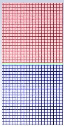
4. Now we are going to open the mesh and we are going to create the mesh of element size of 0.5 mm. Now we are going to update the mesh.
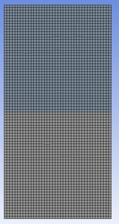
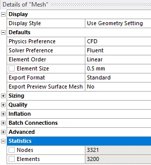
5. Now we are going to setup the case. In the Fluent we will go to Physics. Here we choose the type of solver, we have taken the pressure-based type solver. The Mach number value is less than 0.33 that's why we are using pressure-based solver.
6. Now we have to choose the velocity formulation, we have taken absolute velocity formulation. Now we are going to choose the time, we are using a transient time. Because we want to know that the mixing of the materials with respect to time means how they are going to collapse with respect to time.
7. In this case the gravity is going to play a very important role so we are going to enable it. We are going to give the value of gravity in the Y direction to be -9.81 `m s^-2`. We are going to choose the model to be laminar.
8. Since there are two phases we are going to enable the multiphase. We are going to choose the model to be Volume of Fluid. We are going to use the Implicit Method to solve the simulation.
We want to see the mixing of the fluids at the different-different times and the implicit method is more stable as compared to the explicit method. The explicit method is more time-sensitive and took too much time to calculate so that's why we are going to use the implicit method. So that we can get the answer faster.
9. We want two fluids air and water. So we are going to click on the materials and we are going to add the water in the fluids from the fluent database.
10. We are going to take the time step size to be 0.005 seconds.
11. Now we are going to create the contour plot for the volume fraction. We want the animation for the volume fraction so we are going to create the animation for the volume fraction contour.
12. Now we are going to initialize the value for the calculation. Now we are going to patch the volume to both zones. We want the water in the above zone so we are going to give the volume fraction for water to be 1 and in the below zone we are going to give the volume fraction for water to be 0.
13. Now we are going to start the calculation.
Results
Residual
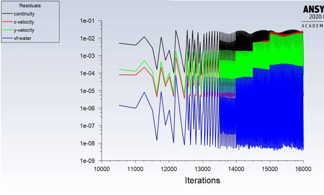
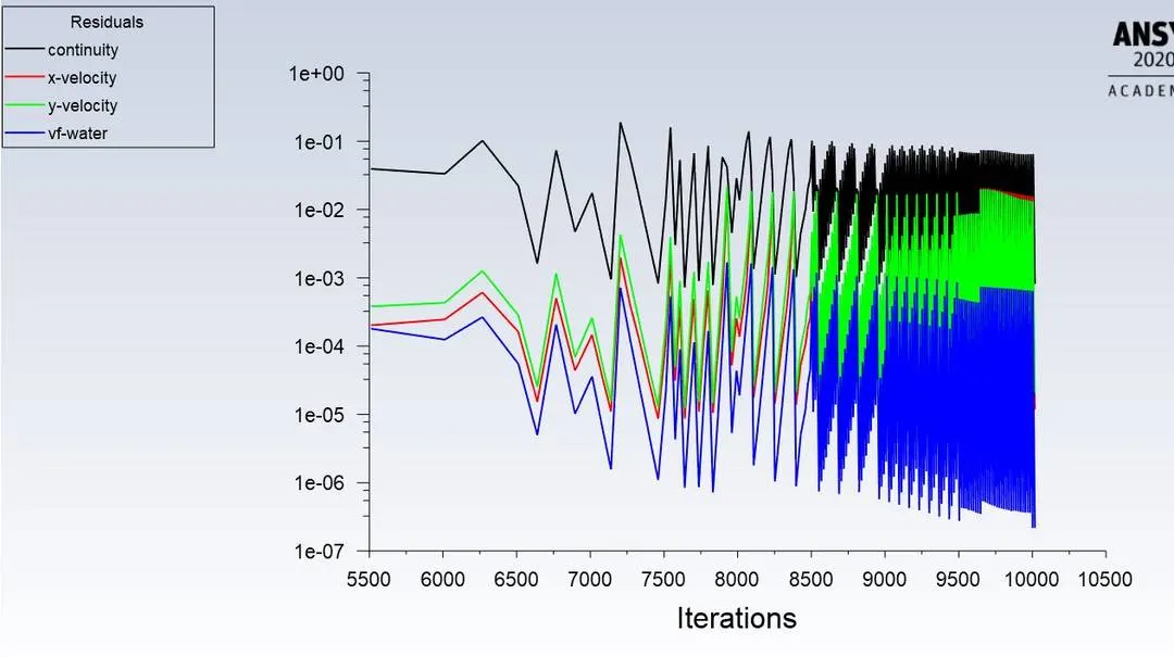
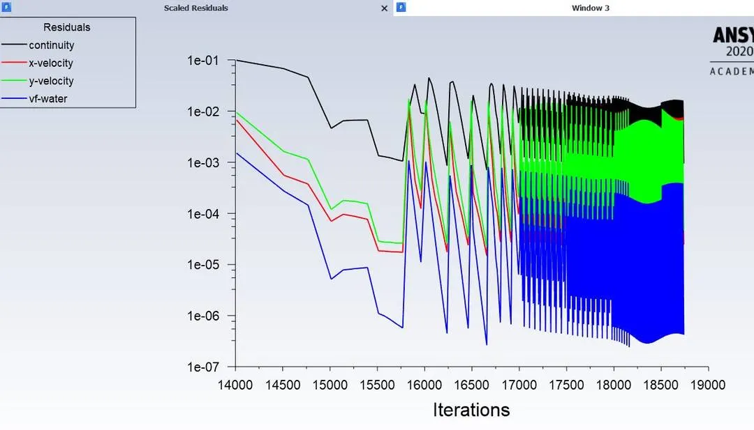
From the residual plot we can see that after some iteration graph is repeating the same pattern. So we can say that we got the converged results.
Animation
After the simulation, we got the following animation:-
https://drive.google.com/file/d/1c9n4jlAtdmDr3p30PRywHKjuLOpQWWHv/view?usp=sharing
Atwood Number
A = `(rho_w-rho_a)/(rho_w+rho_a)`
where
`rho_w` = density of the water = 998.2 `kgm^-3`
`rho_a` = density of the air = 1.225 `kgm^-3`
A = `(998.2-1.225)/(998.2+1.225)=996.975/999.425=0.9975`
Case-2
Finer Mesh
Simulation for water and air.
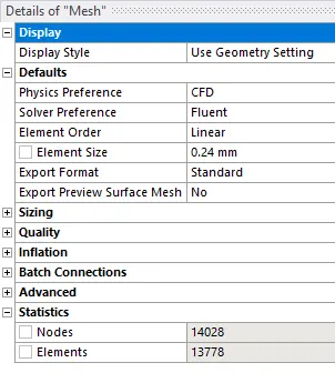
Mesh element size = 0.24 mm
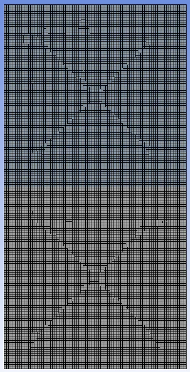
Result
Residuals
Animation
After the simulation, we got the following animation:-
https://drive.google.com/file/d/14rde1rB8QkvPGHvuXFIN7T_eAaeaPont/view?usp=sharing
Atwood Number
A = `(rho_w-rho_a)/(rho_w+rho_a)`
where
`rho_w` = density of the water = 998.2 `kgm^-3`
`rho_a` = density of the air = 1.225 `kgm^-3`
A = `(998.2-1.225)/(998.2+1.225)=996.975/999.425=0.9975`
Case-3
Finer Mesh
Simulation for water and user-defined material.
Mesh element size = 0.24 mm
Changes to be made in the SetUp:-
For the user-defined material, I have copied the water from the fluent database we have to give the following properties:-
Density(`rho`) = 400 `kgm^-3`
Dynamic Viscosity (`mu`) = 0.0001 `kgm^-1s^-1`
Other than those 2 properties we are not going to change any other property. We are going to take the default values for other properties.
Result
Residuals
Animation
After the simulation, we got the following animation:-
https://drive.google.com/file/d/1ofNuNdwi5ia0Qvr23nryq2GR1VNjXcq5/view?usp=sharing
Atwood Number
A = `(rho_w-rho_u)/(rho_w+rho_u)`
where
`rho_w` = density of the water = 998.2 `kgm^-3`
`rho_u` = density of the air = 400 `kgm^-3`
A = `(998.2-400)/(998.2+400)=598.2/1398.2=0.4278`
Comparision
Case-1 Case-2 Case-3
At the beginning (at time step 0)
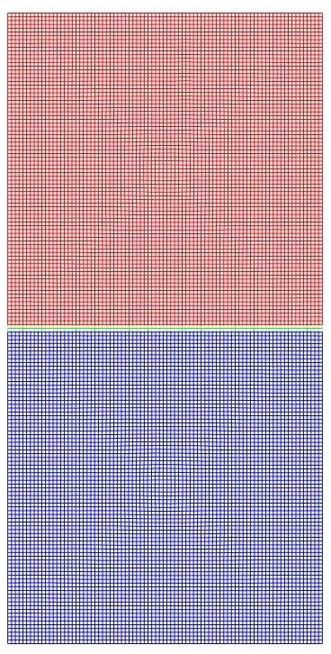
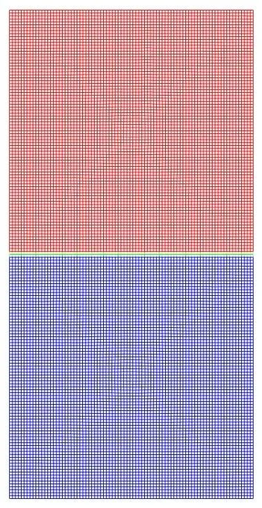
Starting of the Instability
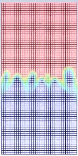
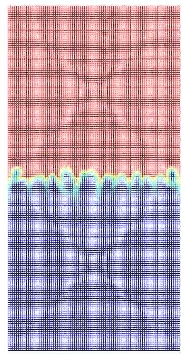
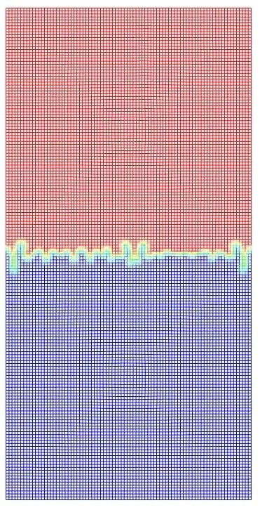
This is the picture when the instability is started and we can see the interface got deformed. For coarse mesh it is happening at iteration number 17, For finer mesh at 9 and for the user-defined mesh (case-3) it is happening at 27 iteration number.
We can see from the picture that the bubble formed in the first two cases is bigger as compared to the third case(less Atwood number).
Big Bubble Formation
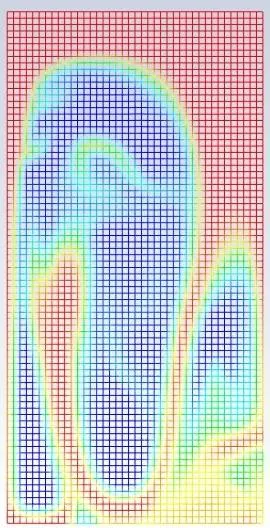
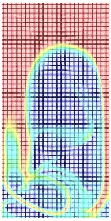
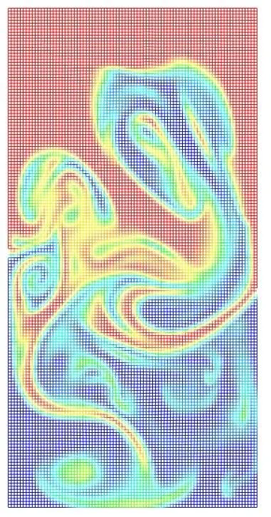
This is the pictures when we get the big bubble. For coarse mesh it is happening at iteration number 48, For finer mesh at 34 and for user defined mesh (case-3) it is happening at 84 iteration number.
We got the big bubble formation in the first two cases we didn't get that big bubble in the third case(less Atwood number).
At time step 198
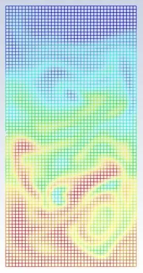
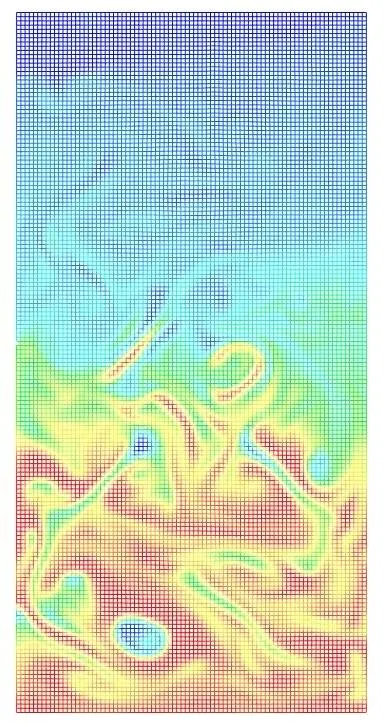
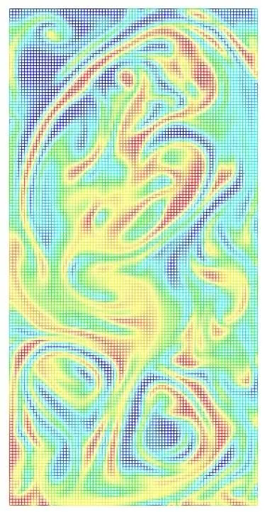
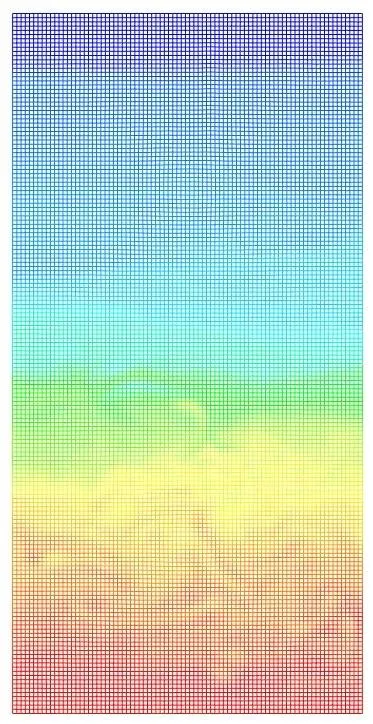
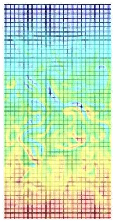
We can see from the picture that instability is more in the case-3, where the Atwood number is low.
At time step 450
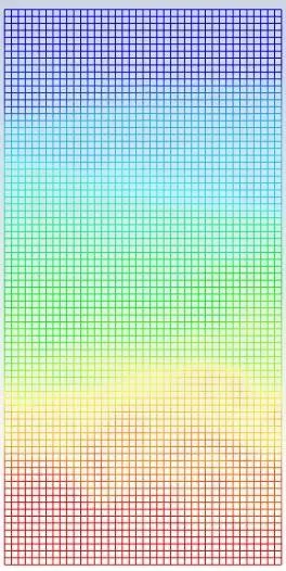
In the end (Final Iteration)
Conclusion
We can see from the above plots that instability is started showing early for the finer mesh.
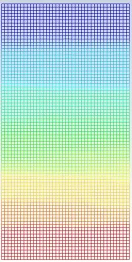
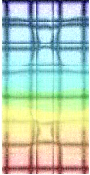
When we use the water and user-defined material instability started late. And to get settle in this case then we have to simulate that for more time as compared to the first two cases.
For the higher Atwood number instability started early.
Higher the Atwood number higher the mixing rate of the materials.
For less Atwood number the materials will take more time to settle down.
When the Atwood number is high, we will get a big bubble when the materials are mixing.
Explain why a steady-state approach might not be suitable for these types of simulations?
The steady-state simulation we do when we are only interested in the result not in how we are getting the answer.
We want to check how the materials are mixing with respect to time. We want to see the instability and how they are mixing every time step so that's why we are using the transient approach.
Transient approach stores the data for every time-step.
I tried to make the mesh more finner so when I take the element size to be 0.1 mm simulation was taking too much time for simulation. So I got the simulation of the water and air until some point and the animation was like this:-
https://drive.google.com/file/d/1jcIAyjF2Y92iMh0iFWAAdM7Vi7wUZnxA/view?usp=sharing