Rayleigh Taylor Instability Challenge

Aim :- Performing Rayleigh Taylor instability between two immiscible liquid.

Theory :-

The Rayleigh–Taylor instability, or RT instability, is an instability of an interface between two fluids of different densities which occurs when the lighter fluid is pushing the heavier fluid. Examples include the behavior of water suspended above oil in the gravity of earth, mushroom clouds like those from volcanic eruptions and atmospheric nuclear explosions, supernova explosions in which expanding core gas is accelerated into denser shell gas, instabilities in plasma fusion reactors and inertial confinement fusion.

Water suspended atop oil is an everyday example of Rayleigh–Taylor instability, and it may be modeled by two completely plane-parallel layers of immiscible fluid, the more dense on top of the less dense one and both subject to the Earth's gravity. The equilibrium here is unstable to any perturburation or disturbances of the interface: if a parcel of heavier fluid is displaced downward with an equal volume of lighter fluid displaced upwards, the potential energy of the configuration is lower than the initial state. Thus the disturbance will grow and lead to a further release of potential energy, as the more dense material moves down under the (effective) gravitational field, and the less dense material is further displaced upwards. This was the set-up as studied by Lord Rayleigh. The important insight by G. I. Taylor was his realisation that this situation is equivalent to the situation when the fluids are accelerated, with the less dense fluid accelerating into the more dense fluid. This occurs deep underwater on the surface of an expanding bubble and in a nuclear explosion.

As the RT instability develops, the initial perturbations progress from a linear growth phase into a non-linear growth phase, eventually developing "plumes" flowing upwards (in the gravitational buoyancy sense) and "spikes" falling downwards. In the linear phase, the fluid movement can be closely approximated by linear equations, and the amplitude of perturbations is growing exponentially with time. In the non-linear phase, perturbation amplitude is too large for a linear approximation, and non-linear equations are required to describe fluid motions. In general, the density disparity between the fluids determines the structure of the subsequent non-linear RT instability flows (assuming other variables such as surface tension and viscosity are negligible here).

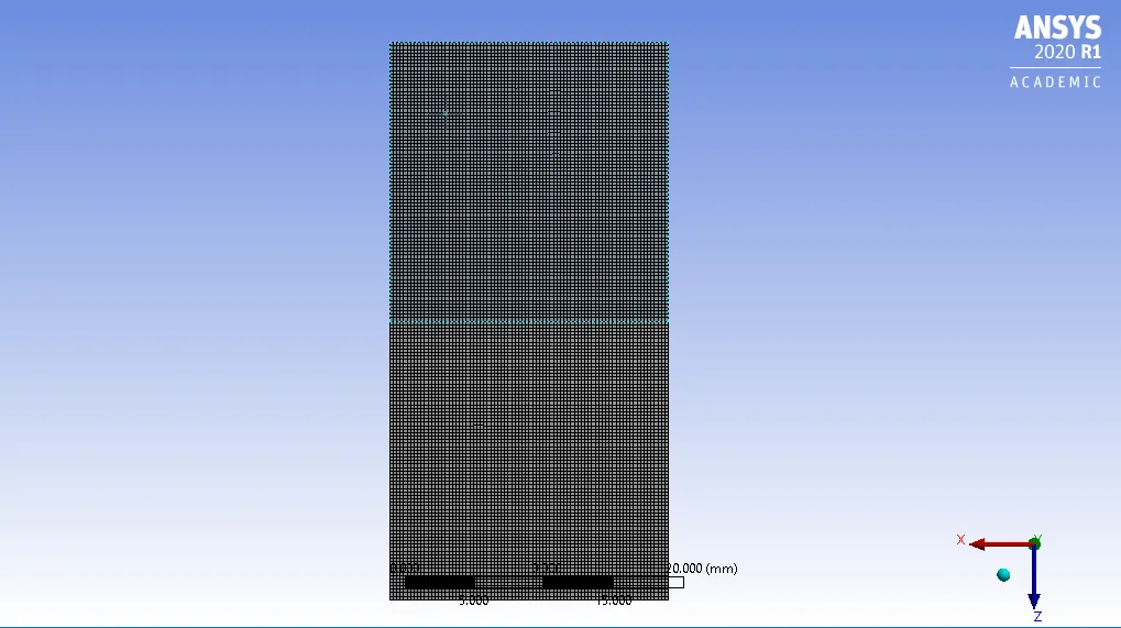
Imported surface in design-modeler with mesh size :-

50mm

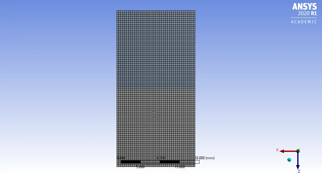
25mm

Preprocessing steps in Ansys fluent :-

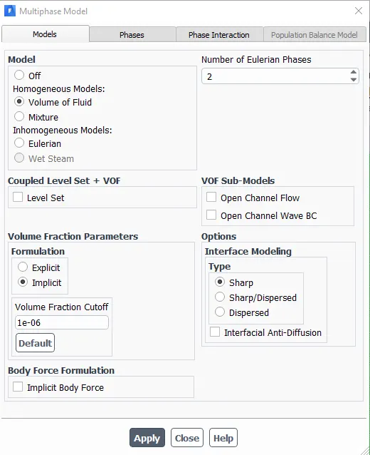
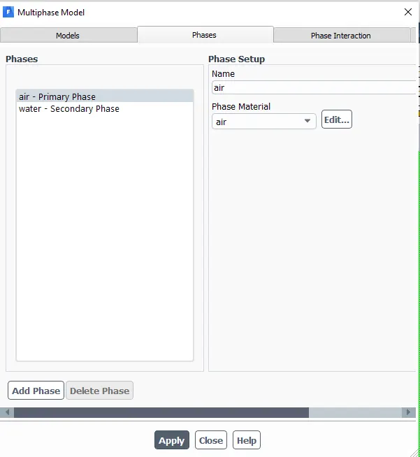
Here We have used multiphase modelling for determining how the flow process take place between the different phases of fluid. The parameters which have been assumed for analysing flow between different phases of fluid have been shown below:-

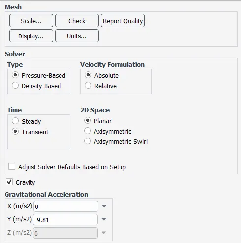
Type of solver used based on time and physical parameter :-

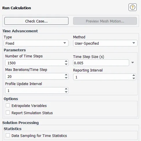
Run calculation parameters :-

Animation of Rayleigh instability for mesh size of 50 mm :-

Animation of Rayleigh instability for mesh size of 25 mm :-

Animation of Rayleigh instability for user defined material :-

The difference in the fluid densities divided by their sum is defined as the Atwood number, A. For A close to 0, RT instability flows take the form of symmetric "fingers" of fluid; for A close to 1, the much lighter fluid "below" the heavier fluid takes the form of larger bubble-like plumes.

The inviscid two-dimensional Rayleigh–Taylor (RT) instability provides an excellent springboard into the mathematical study of stability because of the simple nature of the base state. This is the equilibrium state that exists before any perturbation is added to the system, and is described by the mean velocity field `U(x,z)=W(x,z)=0,\,`where the gravitational field is `g=-ghat z. `An interface at z=0 separates the fluids of densities `rho_G` in the upper region, and `rho_L` in the lower region.`hen the heavy fluid sits on top, the growth of a small perturbation at the interface is exponential, and takes place at the rate.

`exp(gammat)`, with `gamma =sqrt(Agalpha` and A=`(rho_(heavy)-rho_(light))/(rho_(heavy)+rho_(light))`.

Here, in first case of air and water, I see that there was bubble like formation in the shape of plumes from heavier fluid. In this case, I calculated the atwood number and it was as :-

A=`(998.2-1.225)/(998.2+1.225)`= 0.998

Here, in first case of air and water, I see that there was partially bubble and partially finger like formation from heavier fluid. In this case, I calculated the atwood number and it was as :-

A=`(998.2-400)/(998.2+400)` = 0.43 (approx)

So both of our calculations made statement that our simultion is correct.

Here, We cannot use steady state simulation because here We want how the pattern gets create while phases of liquid mixes with each other which we can't be able to obtain in steady state as here We get only final solution. Hence it creates drawback for us hence It become need for us to use transient state where I got the pattern formation at each time-step for overall time-duration.