Rayleigh Taylor Instability Challenge

Rayleigh Taylor Instability

• Problem statement:

1. What are some practical CFD models that have been based on the mathematical analysis of Rayleigh Taylor waves? In your own words, explain how these mathematical models have been adapted for CFD calculations.
2. Perform the Rayleigh Taylor instability simulation for 2 different mesh sizes with the base mesh being 0.5 mm. Compare the results by showing the animations( Attach them from your google drive). Observe the differences in the animation and explain the effect of mesh size on simulation. Also, explain why a steady-state approach might not be suitable for these types of simulation.[ Choose Air and Water for this simulation]
3. Run one more simulation with water and user-defined material(density = 400 kg/m³, viscosity = 0.001 kg/m-s) for refined mesh.
4. Define the Atwood Number. Find out the Atwood number for both the cases and explain how the variation in Atwood number in the above two cases affects the behaviour of the instability.

• Theory:

1. Rayleigh Taylor instability:

The Rayleigh–Taylor instability, or RT instability, is the instability of an interface between two fluids of different densities which occurs when the lighter fluid is pushing the heavier fluid. Examples include the behaviour of water suspended above oil in the gravity of Earth, mushroom clouds like those from volcanic eruptions and atmospheric nuclear explosions, supernova explosions in which expanding core gas is accelerated into denser shell gas, instabilities in plasma fusion reactors and inertial confinement fusion.

Water suspended atop oil is an everyday example of Rayleigh–Taylor instability, and it may be modelled by two completely plane-parallel layers of immiscible fluid, the denser on top of the less dense one and both subject to the Earth's gravity. The equilibrium here is unstable to any perturbations or disturbances of the interface: if a parcel of heavier fluid is displaced downward with an equal volume of lighter fluid displaced upwards, the potential energy of the configuration is lower than the initial state. Thus the disturbance will grow and lead to a further release of potential energy, as the more dense material moves down under the (effective) gravitational field, and the less dense material is further displaced upwards. This was the set-up as studied by Lord Rayleigh. The important insight by G. I. Taylor was his realisation that this situation is equivalent to the situation when the fluids are accelerated, with the less dense fluid accelerating into the more dense fluid. This occurs deep underwater on the surface of an expanding bubble and in a nuclear explosion.

As the RT instability develops, the initial perturbations progress from a linear growth phase into a non-linear growth phase, eventually developing "plumes" flowing upwards (in the gravitational buoyancy sense) and "spikes" falling downwards. In the linear phase, the fluid movement can be closely approximated by linear equations, and the amplitude of perturbations is growing exponentially with time. In the non-linear phase, perturbation amplitude is too large for a linear approximation, and non-linear equations are required to describe fluid motions. In general, the density disparity between the fluids determines the structure of the subsequent non-linear RT instability flows (assuming other variables such as surface tension and viscosity are negligible here). The difference in the fluid densities divided by their sum is defined as the Atwood number, A. For A close to 0, RT instability flows take the form of symmetric "fingers" of fluid; for A close to 1, the much lighter fluid "below" the heavier fluid takes the form of larger bubble-like plumes.

This process is evident not only in many terrestrial examples, from salt domes to weather inversions, but also in astrophysics and electrohydrodynamics. For example, RT instability structure is evident in the Crab Nebula, in which the expanding pulsar wind nebula powered by the Crab pulsar is sweeping up ejected material from the supernova explosion 1000 years ago. The RT instability has also recently been discovered in the Sun's outer atmosphere, or solar corona, when a relatively dense solar prominence overlies a less dense plasma bubble. This latter case resembles magnetically modulated RT instabilities.

Some practical CFD models that have been based on the mathematical analysis of Rayleigh Taylor waves are:

1. Saffman–Taylor instability
2. Richtmyer–Meshkov instability
3. Kelvin–Helmholtz instability
4. Mushroom cloud
5. Plateau–Rayleigh instability
6. Salt fingering
7. Hydrodynamic stability
8. Kármán vortex street
9. Fluid thread breakup

2. Atwood number:

The Atwood number (A) is a dimensionless number in fluid dynamics used in the study of hydrodynamic instabilities in density stratified flows. It is a dimensionless density ratio defined as

where

= density of heavier fluid

= density of lighter fluid

• Geometry setup:

1. Choose Fluent from the workbench setup, edit spaceclaim to create geometry.

2. Choose the XY plane to sketch 2D the geometry, create a square of 20mm and select pull tool to make it as surface.

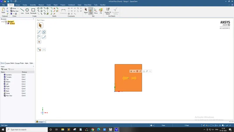
3. Move the geometry to new component and rename its as Air.

4. Now create new geometry under the same component as air geometry and create a square of 20mm right on top of air square which creates a interface between the 2 boxes. And name this box as water.

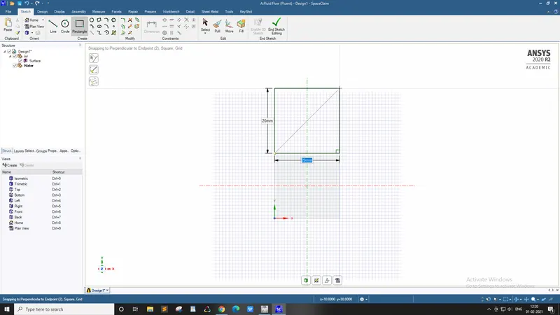
5. Select the entire geometry for share prep under workbench and select share so that the interface can face information and conformal meshing can be achieved between the 2 phases.

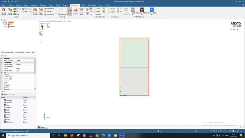
6. Check the main geometry properties and set to share topology and now we can close space claim and move ahead with meshing.

• Meshing setup:

1. After creating the geometry, generate a base mesh of 0.5mm since the geometry is very simple and does not require much cells and later refine for further simulations.

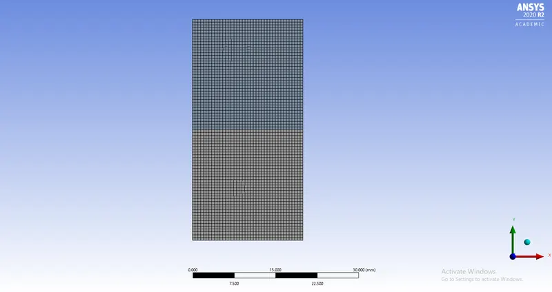
2. close meshing and move ahead with fluent.

• Fluent setup:

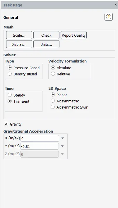
1. Set the general settings to pressure based solver, absolute velocity and transient state simulation because we are interested with knowing the physical changes of mixing of 2 phase fluids wrt time. select gravity and enter the value in the Y- axis so that the denser fluid is pulled down due to gravity.

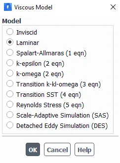
2. Under Physics drop down, choose laminar model, multiphase discretisation method.

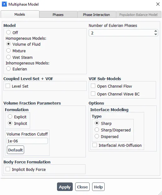
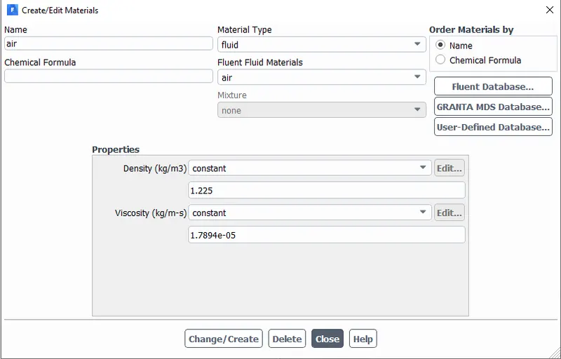
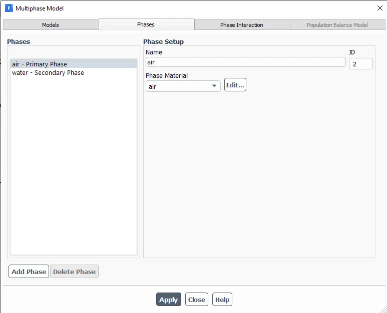
3. Add materials, copy water and air as primary(air) and secondary(water). Now go back to multiphase model and under phase, assign the primary and secondary phases.

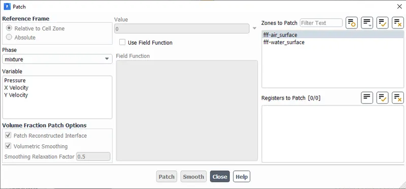
4. Intialise using the standard initialisation and use the patch command to assign the aplha value of each phase, water as 1 and air as 0.

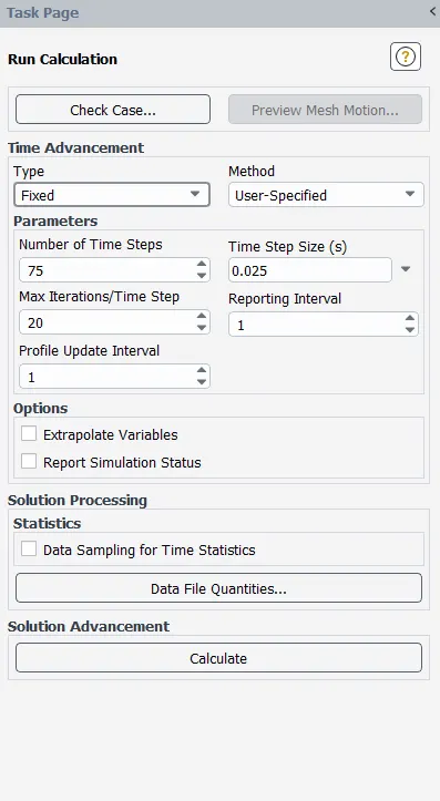
5. Run the simulation by assigning a proper time step size and number of iterations so that the fluid is nicely settled in the end.

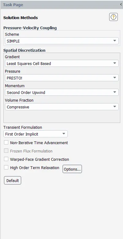
6. If an error is encountered due to divergence, try to reduce the solution controls accordingly.

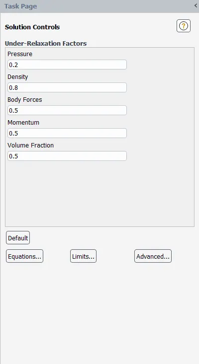
7. create contours and other output plots to view the mixing of 2 fluids.

• CFD post:

1. Use the CFD post to view the animation by creating contour planes and view the fluid motion between the 2 phase geomteries.

2. After saving the animation on fluent, CFD post can be used to save the animation clip which can be viewed using any media supported applications.

• Results:

The simulation is run for 3 different settings,

a. Base mesh of 0.5mm having the fluid materials as water and air.

b. Refined mesh of 0.17mm having the fluid materials as water and air.

c. Refined mesh of 0.17mm having the fluid materials as water and user-defined material having density= 400 kg/m^3 and viscosity= 0.001 kg/m-s.

1. Base mesh:

Element size= 0.5mm

No. of elements= 3200

Time step size= 0.025

No. of iterations= 100

• Mesh:

• Plots:

1. Residuals:

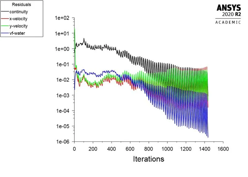
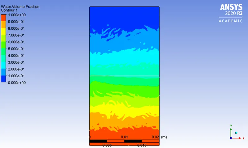
2. Mixing Final mesh contour:

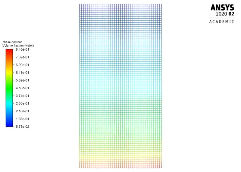
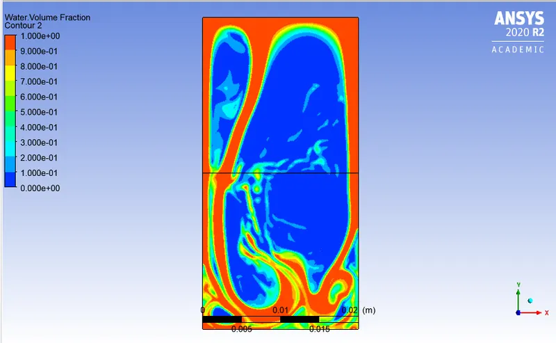
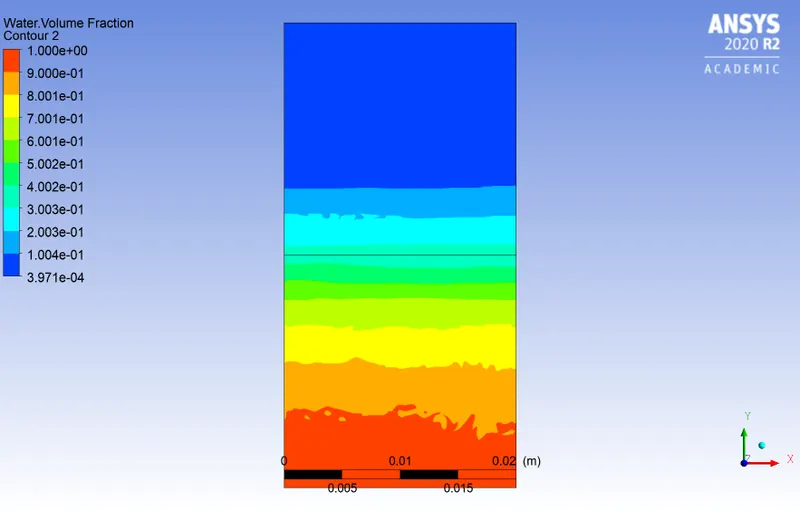
2. Refined mesh:

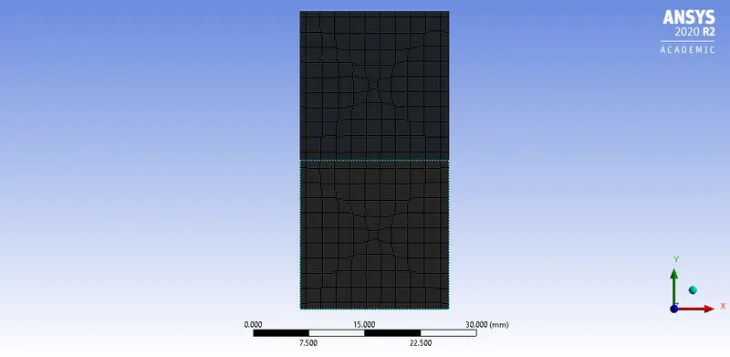
Element size= 0.17mm

No. of elements= 27848

Time step size= 0.001

No. of iterations= 400

• Mesh:

• Plots:

1. Residuals:

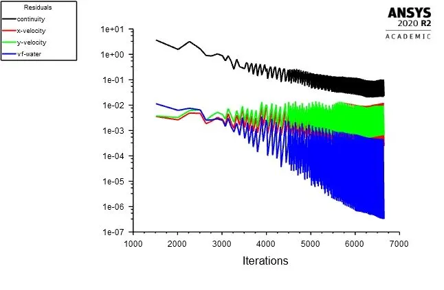
2. Mixing final mesh contour:

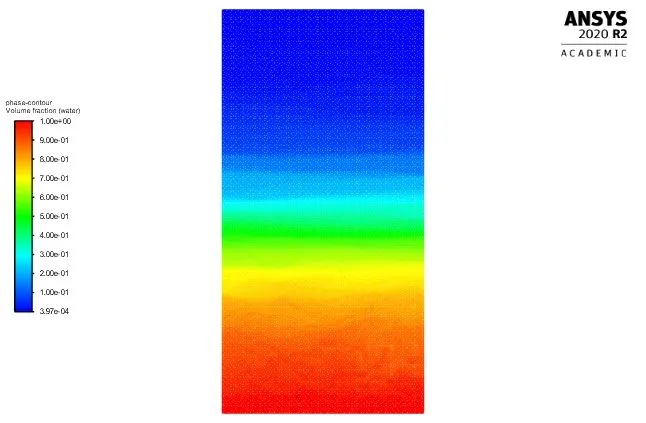
3. CFD post contours:

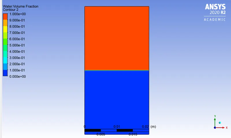
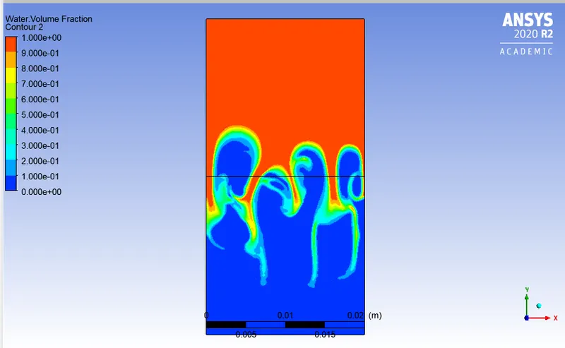
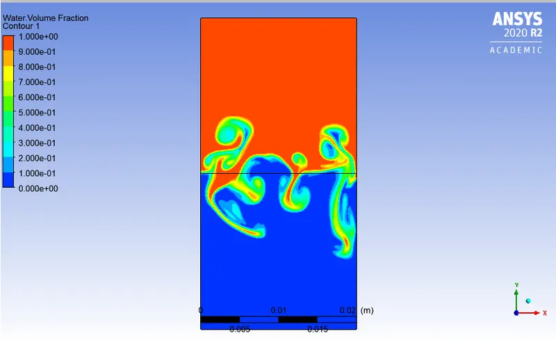
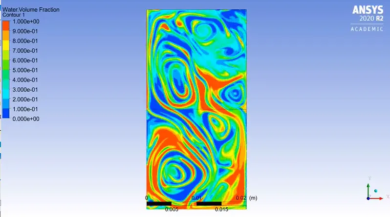
3. Refined mesh with user-defined material and water:

Element size= 0.17mm

No. of elements= 27848

Time step size= 0.001

No. of iterations= 400

• Mesh:

• Plots:

1. Residuals:

2. Mixing final mesh conotur:

3. CFD post contours:

• Output animations googe drive links:

1. Base mesh : https://drive.google.com/file/d/1f6XVRYIVXxGQw-EWTyI_SweURAnNmVja/view?usp=sharing

2. Refined mesh: https://drive.google.com/file/d/1InlHwtqQP5CP62jtHda2PcrWdKzWoOrW/view?usp=sharing

3. User-defined: https://drive.google.com/file/d/1QynG1_5NXmA3VODiTw84jMurdvk4pzRH/view?usp=sharing

• Discussions and conclusions:

Calculating Atwood number:

Atwood number (Air -water) = (998.2-1.225)/ (998.2+1.225) = 0.9975.

Atwood number (User defined material -water) = (400-1.225)/ (400+1.225) = 0.9938.

As in our solution we see that the lighter fluid rises up and bubble formation takes place. The atwood number calculated in our case is almost close to 1. Hence it signifies that both obtained simulation result and the atwood calculation results are same , thus validates the results.

• Conclusions:

1. On running multiple simulations Rayleigh Taylor Instability was observed at the interface of the fluids with different densities under the influence of the gravity.
2. It is clear that the lower density fluid is setteled on top and the higher density fluid is settled at the bottom. This is formed because of the instability.Slowly these instabilities start growing which is calle as Rayleigh Taylor Instability.
3. Also observed that the instabilites are slowly forming into individual bubbles, which replaces the position of fluids.
4. By performing different set of mesh refinement it is clear that on refining to the fine mesh the simulation is much better when compared with the baseline mesh.
5. The instabilities that are happening at the interface is clearly visualized as we refined the mesh quality.
6. Compared to initial simulations, in the last case the irregularities are more clear in the form of bubbles and the formation of vortices are also clear in this case.
7. As the grid siize is much fine , predicting the flow is more accurate and clear for visualization.
8. In the initial stages , we noticed that time step affecting the flow formation. Hence selecting the time step is also important to save the computation time.
9. On running multiple simulations Rayleigh Taylor Instability was observed at the interface of the fluids with different densities under the influence of the gravity.