Standard Rankine Cycle Simulation using Matlab

A Rankine cycle is a type of steam cycle in which the working fluid is water, which is sometimes in the liquid phase and sometimes in the vapour phase during its cycle of operation. In this cycle, each process is assumed to be an ideal process, i.e., an idealised thermodynamic cycle of a heat engine that converts heat into mechanical work.

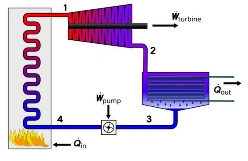
Below is an illustration of a basic Rankine cycle.

Boiler

In the boiler, steam is generated by reversible isobaric heating of water. It will produce super-heated steam.

Steady flow energy equation (SFEE) for the boiler (as control volume):

`h_4 + Q_1 = h_1 => Q_1 = h_1 - h_4`

where Q is heat and h is enthalpy.

Turbine

In a steam turbine, the reversible adiabatic expansion of steam takes place. It will produce mechanical work.

SFEE of the turbine (as control volume):

`W_(turb) = h_1 - h_2`

where W is work.

Condenser

In the steam condenser, there would be reversible isobaric heat rejection till the steam converts into saturated liquid.

SPEE of condenser:

`Q_(cond) = h_2 - h_3`

Pump

In the pump, the saturated liquid is compressed and reversible adiabatic ending at an initial pressure. It pumps the water to the boiler.

SFEE of pump: (ds = 0)

`W_(pump) = h_4 - h_3`

Hence,

The net-work done by the cycle is, `W = W_(turb) - W_(pump)`

The efficiency of the Rankine cycle

`eta = W/Q_1`

Aim: To create a Rankine cycle simulator using Matlab.

Objectives:

1. Calculate the thermodynamic properties at each state point of the Rankine cycle based on user input.
2. Plot the T-S and H-S plots for each simulation.
3. Calculate the net-work output and back work ratio.
4. Save the output in the command window to a text document.

Here is the link to the steam table library used for this project: XSteam Library

Main Code

close all
clear global
clc

%% User inputs
fprintf('RANKINE CYCLE SIMULATOR\n\n')
p1 = input('Enter the pressure at the TURBINE INLET (in bar): p1 = '); % Pressure of super-heated steam
t1 = input('Enter the TEMPERATURE at the TURBINE INLET (in Celcius): t1 = '); % Temperature of super-heated steam
p2 = input('Enter the PRESSURE at the CONDENSER (in bar): p2 = '); % Pressure of wet steam
fprintf('\n\n')

filename = "p1="+p1+" t1="+t1+" p2="+p2+".txt";
if not(isfile(filename))
    diary(filename)
else
    res = input('This simulation was run and this report exists. Would you like to delete this and re-create a new one? (Y/N) ');
    fprintf('\n');
    if res == 'Y'
        delete(filename)
        diary(filename)
    end
end
diary(filename)

%% OUTPUT DESCRIPTION

fprintf('RANKINE CYCLE SILULATION RESULTS\n');
fprintf('Process 1-2: Isentropic Expansion of vapor in the Turbine\n');
fprintf('Process 2-3: Isobaric Heat Rejection from the condenser\n');
fprintf('Process 3-4: Isentropic Compression at the pump\n');
fprintf('Process 4-1: Isobaric Heat Addition by the Boiler\n\n');

%% STATE Calculations
disp('RESULTS')
fprintf('\n');

% State 1: Boiler output and turbine input: 
% Superheated steam
disp('STATE 1: Superheated steam: Boiler output')
fprintf('Pressure = %f bar\n',p1);
fprintf('Temperature = %f C\n',t1);
s1 = XSteam('s_pT',p1,t1); fprintf('Specific entropy = %f KJ/(kg C)\n',s1); % Returns saturated vapour entropy if mixture
h1 = XSteam('h_pT',p1,t1); fprintf('Enthalpy = %f KJ/Kg\n\n',h1); 

% State 2: Turbine output and condenser input: Work output from turbine
% Wet steam
% This state point doesn't lie on the saturation curve. Its lies within 0 and 1, more close to 1
disp('STATE 2: Wet steam: Turbine output')
fprintf('Pressure = %f bar\n',p2);
s2 = s1; fprintf('Specific entropy = %f KJ/(kg C)\n',s2);
t2 = XSteam('Tsat_p',p2);
%t2 = XSteam('T_ps',p2,s2); 
fprintf('Temperature = %f C\n',t2); % Temperture as a function of pressure and entropy

sf2 = XSteam('sL_p',p2); % Saturated liquid entropy
sg2 = XSteam('sV_p',p2); % Saturated vapour entropy
hf2 = XSteam('hL_p',p2); % Saturated liquid enthalpy
hg2 = XSteam('hV_p',p2); % Saturated vapour enthalpy

X2 = (s2-sf2)/(sg2-sf2); fprintf('Dryness fraction = %f\n',X2); % Dryness fraction of wet steam
h2 = hf2 + X2*(hg2-hf2); fprintf('Enthalpy = %f KJ/Kg\n\n',h2); % Specific Enthalpy at state 2


% State 3: Condenser output and pump input
% Saturated liquid 
disp('STATE 3: Saturated Liquid: Condenser output')
t3 = t2; fprintf('Temperature = %f C\n',t3); % Temperature of saturated liquid
p3 = XSteam('psat_T',t3); fprintf('Pressure = %f bar\n',p3); % Pressure of saturated liquid
s3 = XSteam('sL_p',p3); fprintf('Specific entropy = %f KJ/(kg C)\n',s3); % Saturated liquid entropy
h3 = XSteam('hL_p',p3); fprintf('Enthalpy = %f KJ/Kg\n\n',h3); % Saturated liquid enthalpy

% State 4a: Pump output
% Subcooled liquid
disp('STATE 4: Sub-cooled liquid: Pump output')
s4 = s3; fprintf('Specific entropy = %f KJ/(kg C)\n',s4);
p4 = p1; fprintf('Pressure = %f bar\n',p4);

cp4 = XSteam('CpL_p',p3); % Specific isobaric heat capacity as a function of pressure and entropy.
cv4 = XSteam('CvL_p',p3); % Specific isochoric heat capacity as a function of pressure and entropy.
Y = cp4/cv4;
expo = (Y-1)/Y;

t4 = t3*(p4/p3)^expo; fprintf('Temperature = %f C\n',t4); % Temperature of liquid at pump outlet
h4 = XSteam('h_ps',p4,s4); fprintf('Enthalpy = %f KJ/Kg\n\n',h4); % Enthalpy of liquid at pump outlet

% State 4a: Exactly at the boiler input
% Saturated liquid
disp('STATE 4a: Saturated Liquid: Boiler input')
p4a = p4; fprintf('Pressure = %f bar\n',p4a);
s4a = XSteam('sL_p',p4a); fprintf('Specific entropy = %f KJ/(kg C)\n',s4a); % Saturated liquid entropy as a function of pressure
t4a = XSteam('Tsat_p',p4a); fprintf('Temperature = %f C\n',t4a); % Saturation temperature
h4a = XSteam('hL_p',p4a); fprintf('Enthalpy = %f KJ/Kg\n\n',h4); % Saturated liquid enthalpy as a function of pressure

% State 1a: inside the boiler
% Saturated vapour
disp('STATE 1a: Saturated Vapour: Inside the boiler')
t1a = t4a; fprintf('Temperature = %f C\n',t1a);
p1a = p4; fprintf('Pressure = %f bar\n',p1a);
s1a = XSteam('sV_p',p1a); fprintf('Specific entropy = %f KJ/(kg C)\n',s1a);
h1a = XSteam('hV_p',p1a); fprintf('Enthalpy = %f KJ/Kg\n\n',h1a);

%% PROCESS CALCULATIONS
disp('WORK DONE AND HEAT TRANSFER RESULTS')
fprintf('\n');

% Process 1 - 2: Icentropic expansion of vapour in the turbine 
W_turb = h1 - h2; fprintf('Work done by turbine = %f KJ/Kg\n',W_turb);

% Process 2 - 3: Isobaric heat rejection from the condenser
Q_cond = h2 - h3; fprintf('Heat rejection by condenser = %f KJ/Kg\n',Q_cond);

% Process 3 - 4: Icentropic compression of the pump
W_pump = h4 - h3; fprintf('Work done by pump = %f KJ/Kg\n',W_pump);

% Process 4 - 1: Isobaric heat addition by boiler
Q_boil = h1 - h4; fprintf('Heat injection by boiler = %f KJ/Kg\n',Q_boil);

% Net-work done by the cycle
W_net = W_turb - W_pump; fprintf('Net work done by the cycle = %f KJ/Kg\n',W_net);

% Back work ratio
BWR = W_pump/W_turb; frpintf('Back work ratio = %f\n',BWR);

% Effeciency of the Ranking cycle
rankcyc_eff = W_net*100/Q_boil; fprintf('Effeciency of this rankine cycle = %f percent\n',rankcyc_eff);

SSC = 3600/W_net; fprintf('SSC = %f Kg/KJ\n\n',SSC);

if res == 'Y'
    diary off
end

%% PLOTTING
ct = 373.9;
T_range = linspace(0,ct,ct*100);
sat_liq_curv_s = zeros(); sat_vap_curv_s = zeros();
sat_liq_curv_h = zeros(); sat_vap_curv_h = zeros();
for i = 1:length(T_range)
    sat_liq_curv_s(i) = XSteam('sL_T',T_range(i));
    sat_vap_curv_s(i) = XSteam('sV_T',T_range(i));
    sat_liq_curv_h(i) = XSteam('hL_T',T_range(i));
    sat_vap_curv_h(i) = XSteam('hV_T',T_range(i));
end

crtp_s = sat_liq_curv_s(end) + (sat_vap_curv_s(end) - sat_liq_curv_s(end))/2;
crtp_h = sat_liq_curv_h(end) + (sat_vap_curv_h(end) - sat_liq_curv_h(end))/2;

T = [t1 t2 t3 t4 t4a t1a];
S = [s1 s2 s3 s4 s4a s1a];
H = [h1 h2 h3 h4 h4a h1a];

% TS Curve

figure()
plots(S,T,"Temperature (C)",sat_liq_curv_s,sat_vap_curv_s,T_range,T_range,crtp_s,ct)

% HS Curve or Mollier diagram

figure()
plots(S,H,"Enthalpy (KJ/Kg)",sat_liq_curv_s,sat_vap_curv_s,sat_liq_curv_h,sat_vap_curv_h,crtp_s,crtp_h)

Main code explanation:

• Line 7-9: The values of p1, t1 and p2 are collected from the user using the input() function.
• Line 12-22: A Text document of the report is created.
  
  • the filename is the name of the report.
  • If the file doesn't exist, record it in it using the diary function, which will read the contents in the command window.
  • If the file exists, delete the existing file and create a new one and start recording.
• Line 36-99: State calculations
  
  • How to access the XSteam library:
    • XSteam('Property name',inputs,inputs)
      • The characters at the end of the underscore in the property name define the inputs it requires. For example, 's_pT' means it will return the value of specific entropy upon providing the pressure and temperature values.
  • Line 54 - 60
    • Dryness fraction at state 2, `x_2 = (s_2 - s_(f2))/(s_(g2) - s_(f2))`
    • The enthalpy at state 2, `h_2 = h_(f2) + x_2*(h_(g2)-h_(f2))`
• Line 102 - 130: Process calculations
• Line 133 - 159: Plots
  • Line 133: ct = critical temperature: The maximum temperature the Xsteam library can take.
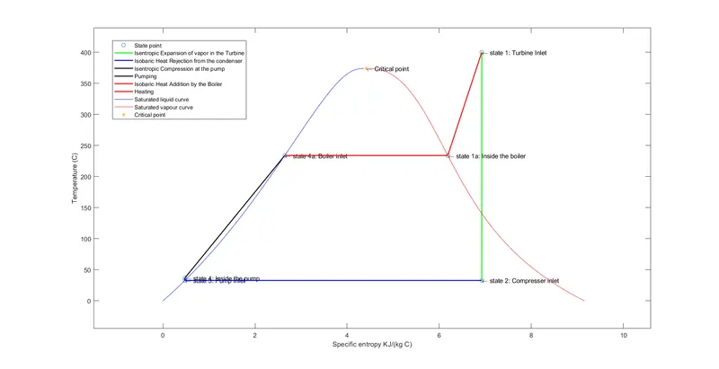
  • Line 154: Calling the plots function and plotting the TS plot
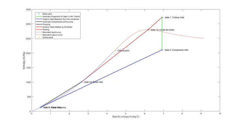
  • Line 159: Calling the plots function and plotting the HS plot

Plotting function:

function plots(x,y,yname,ccx,ccy,ccz,ccza,crx,cry)
    plot(x,y,'o')
    statelables(x,y);
    xlabel('Specific entropy KJ/(kg C)')
    ylabel(yname)
    hold on
    plot([x(1) x(2)],[y(1) y(2)],'Linewidth',1.5,'Color','g')
    plot([x(2) x(3)],[y(2) y(3)],'Linewidth',1.5,'Color','b')
    plot([x(3) x(4)],[y(3) y(4)],'Linewidth',1.5,'Color','k')
    plot([x(4) x(5)],[y(4) y(5)],'Linewidth',1.5,'Color','k')
    plot([x(5) x(6)],[y(5) y(6)],'Linewidth',1.5,'Color','r')
    plot([x(6) x(1)],[y(6) y(1)],'Linewidth',1.5,'Color','r')
    plot(ccx,ccz,'Color','b')
    plot(ccy,ccza,'Color','r')
    plot(crx,cry,'*')
    text(crx,cry,'\leftarrow Critical point')
    legend('State point','Isentropic Expansion of vapor in the Turbine','Isobaric Heat Rejection from the condenser','Isentropic Compression at the pump','Pumping','Isobaric Heat Addition by the Boiler','Heating','Saturated liquid curve','Saturated vapour curve','Critical point')
end

Results:

Simulation results in the command window:

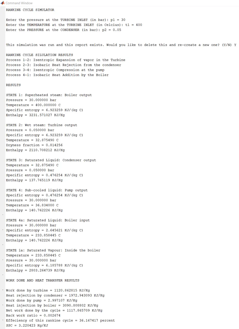
Temperature vs Entropy plot:

Enthalpy vs Entropy plot:

Errors faced during the development of the code:

Fortunately, no errors were faced during the code.