Project - Speed Control of a Direct Current (DC) motor

1. In this project, a Simulink model for the DC motor will be first developed per the schematic shown in Figure 1.

Here we take the motor parameters as,

Here we observe that, the real part of the poles is negative, so the poles lie in the left half of the jw plane & hence the system is stable.

The Kp & Kd values are 13.1892 & -0.348 respectively

Kp=13.1892

Kd=-0.348

Now we build the model as:

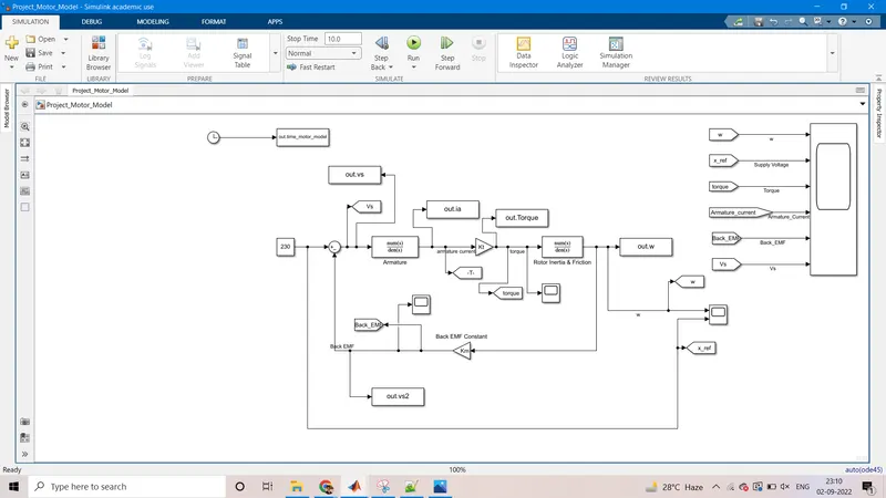
We use multiple gain, sum , transfer function blocks with an integrator block & a constant block which acts as the input to the entire system. The value of the constant block is taken as 230 units.

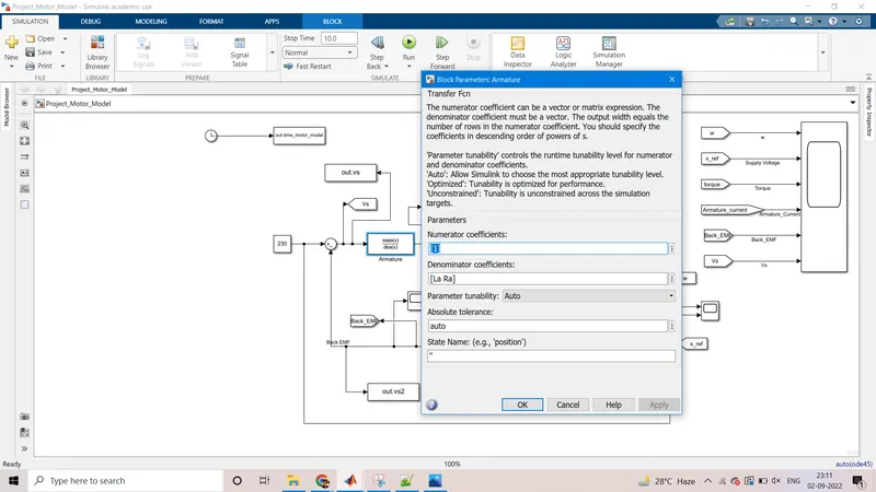
The armature block is composed of the parameters La & Ra from the workspace

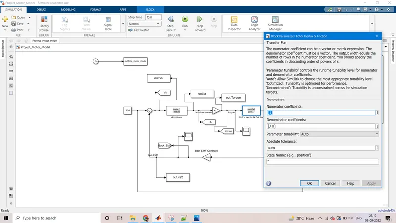
The rotor block is composed of the parameters J & H from the workspace

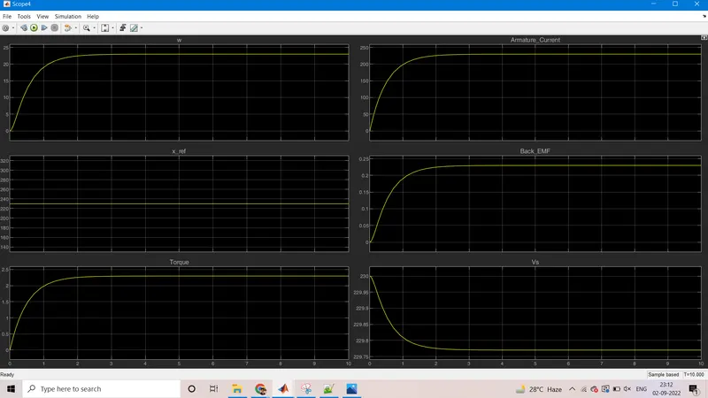
Here we observe that the speed has the same nature as the reference signal , but lacks in magnitude due to the absence of speed control, which we accomplish in the next step. The supply voltage reamins constant at 230V. Torque, back emf & current all have the nature identical to the reference signal & settle at a constant value in a short period of time. Vs begins a higher value of 230V & recedes to a constant value 229.7875V with time.

Hence the mathematical model of a dc motor is created & it performs accurately.

2. Use the Proportional, Integral, and Derivative (PID) control design knowledge gained in the training to design, develop and test a controller to maintain a desired speed for the motor.

Here we take the motor parameters same as above,

Here we observe that, the real part of the poles is negative, so the poles lie in the left half of the jw plane & hence the system is stable.

The Kp & Kd values are 13.1892 & -0.348 respectively

Kp=13.1892

Kd=-0.348

Now we build the model by making some modifications in the previous case as:

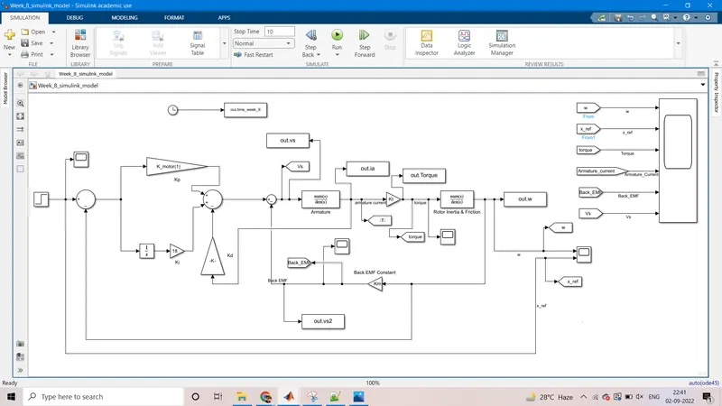
We use multiple gain, sum , transfer function blocks with an integrator block & a step function which acts as the input to the entire system. After trying multiple values for Ki, we choose the value of 18 as it provides the best & accurate response for the given parameters.

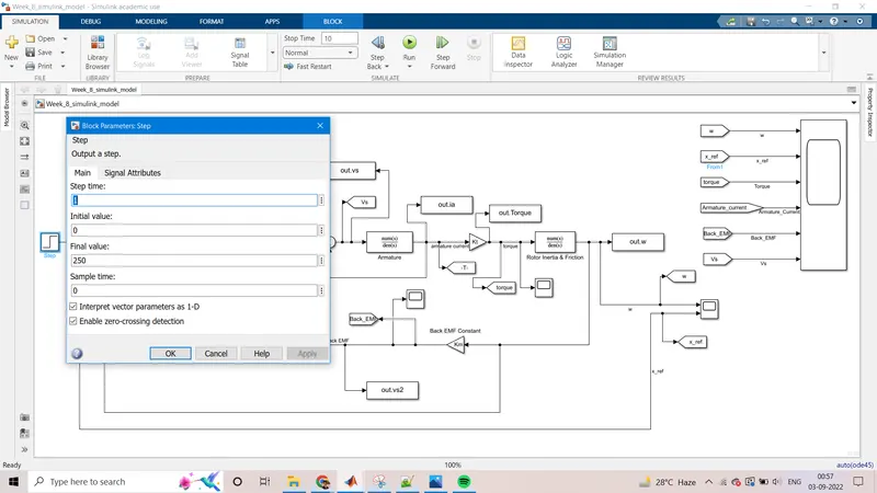
The step function has a step time of 1 second, intial value of 0 & final value of 250.

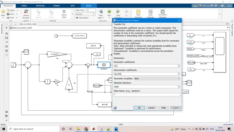
The armature block is composed of the parameters La & Ra from the workspace

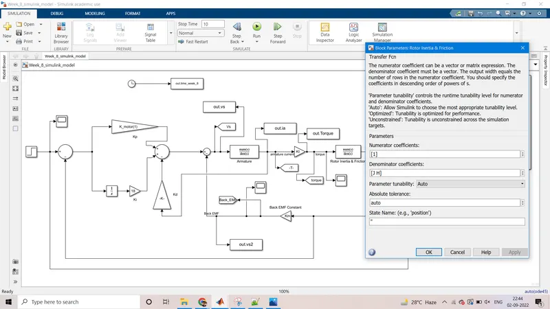
The rotor block is composed of the parameters J & H from the workspace

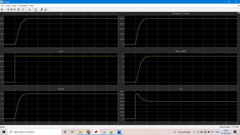
We observe the plot for all 6 parameteers.

The speed follows the reference value with some lag, with optimal settling time & eventually settles at the value of 250 as desired.

The armature current follows the nature of the step function & attain a high value of 2500A

The back emf has the same nature as the reference signal & settles at 2.5V

The Torque has the same nature as the input signal & settles at 25 Nm

Vs has the same nature as the reference signal & settles at 2500V after some overshoot initially.

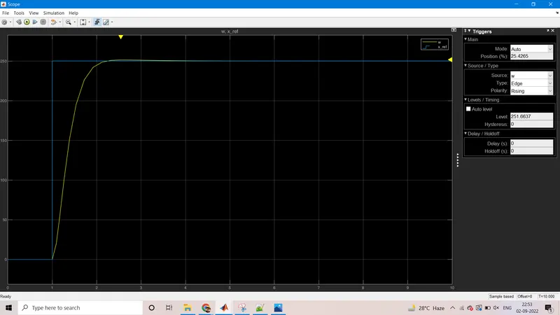
Here we observe that the at the highest point for the speed signal w is at 251.66 which is way below the limit of 5% overshoot (5% would be at 262.5), Hence the condition for overshoot error being less than 5% is satisfied. We also observe that the signal w reaches the reference value of 250 well within 2 seconds from its ascend & hence we conclude that the settling time is less than 2 seconds. The response signal coincides with the refernece speed after the system stablizes & the difference between the desired value & the output value is 0 & hence the steady state error is 0% (<1%).

Hence all three control design objectives are satisfied & the system performs the control function accurately.

%Motor speed control matlab script
J=0.01;
H=0.1;
Km=0.01;
Kt=0.01;
Ra=1;
La=0.5;
zeta_8=0.9;
A_motor=[-H/J Kt/J; -Km/La -Ra/La];
B_motor=[0;1/La];
p1=-zeta_8*wn+wn*sqrt(zeta_8^2-1);
p2=-zeta_8*wn-wn*sqrt(zeta_8^2-1);
P_motor=[p1 p2];
K_motor=place(A_motor,B_motor,P_motor);

(Note: For the model we used fixed step discrete solver with ode4 method (Runge Kutta method) with a step size of 0.01s)