Project - Speed Control of a Direct Current (DC) motor
Mathematical modeling of the system:
A mathematical model of a dynamic system is defined as a set of equations that represents the dynamics of the system. The dynamics may be obtained by using physical laws governing a particular system.
Step 1: Obtaining differential equations using physical laws
Modeling a direct current machine:
Direct current (DC) machines can function as a generator or motor. A DC machine has a rotor that is the rotating part with an armature winding providing the electrical circuit. It also has as data that is the stationary part with the field winding serving as a magnet when energized
Generator mode:
While operating in generator mode, a prime mover is coupled to the rotor, allowing it to rotate in the magnetic field created by the field winding. Mechanism and electromotive force (EMF) in the conductor mounted on the rotor contributes to voltage generation.
Motor mode:
While operating in motor mode the electrical energy supplied to the armature winding and the field winding contributes to the rotating magnetic field that forces the rotor to rotate which generates mechanical torque.
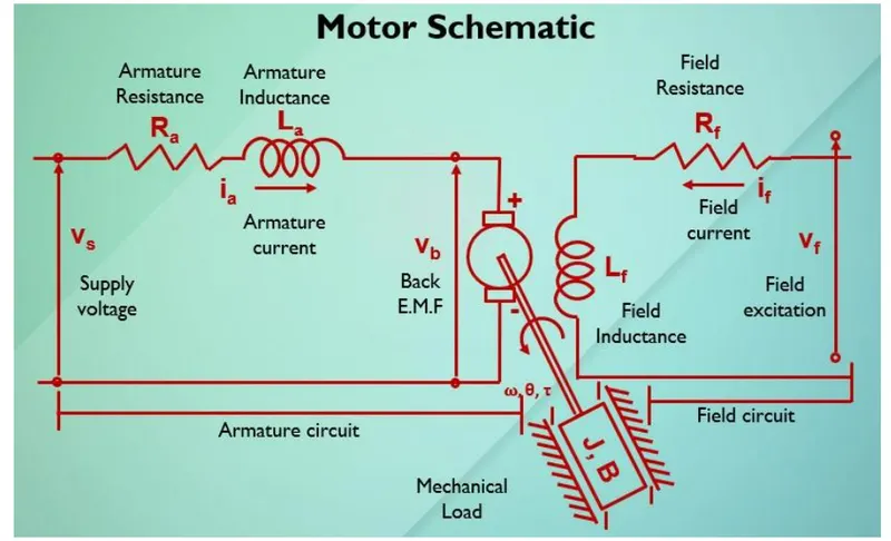
Parameters in DC Motor:
J - Moment of Inertia of Rotor in kg-m^2
B - Motor viscous friction constant in N-m-s
Km- Back emf constant in v/rad/s
Kt- Torque constant in N-m/amp
Ra- Armature Resistance in ohms
La- Armature Inductance in henries
Using Kirchhoff's Voltage law,

As per Newton's law

Step 2: Converting the obtained equations to S domain

By keeping I(s) on LHS, we get


By Keeping w(s) on LHS, we get

Substitute I(s) value to equation (5), we get




Step 3: Obtaining Transfer function using Laplace Transform
Transfer function:
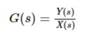
Transfer functions are used to characterize the input-output relationship of components
or systems that can be described by differential equations. Transfer function is the ratio
of Laplace transformed output to the Laplace transformed input and all initial conditions
are zero. Using the concept of transfer function, the dynamic system is represented by
an algebraic equation in S Domain.
where
Y(S)-Laplace transformed output
X(S)-Laplace transformed input
Transfer function of DC Motor:

Where ,
w(s) is the angular velocity - output of motor
V(s) is the supply voltage - input of motor
Step 4: Converting Transfer function to state space equations
Intial conditions are zero for the transfer function, we need to convert
them into state space equations for analysing system behaviour with
different initial condions.
State space representation:
Any linear differential equation can be cast in a state space representation
with input output and the state variables that are related by first order
differential equations.
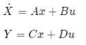
If we use Matrix form notation to represent these two first order differential
equation is called state space representation of the dynamic system and is
generally shown as:
where,
X is the state vector (nx1)
Y is the output equation (mx1)
U is the input vector(rx1)
A is this state matrix(nxn)
B is the input matrix(nxm)
C is the output matrix(Pxn)
D is the feedforward matrix(qxp)
State space equation for the DC Motor:

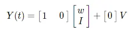
Correlation between transfer function and state space equations:
MATLAB has functions to convert a state space system into a transfer function
with numerator and denominator polynomials and vice versa.
ss2tf and tf2ss
Syntax:
[NUM,DEN] = ss2tf(A,B,C,D,iu)
[A,B,C,D] = tf2ss(NUM,DEN)
Where A, B, C and D are the state space Matrices
NUM and DEN vectors contain the coefficients of the numerator and the
denominator polynomials. The transfer function is derived from Eigenvalues of a
matrix A are the same as the poles of the transfer function. They are obtained from
solving the determinant also called the characteristic equation.
PID Controller:
The equation for the output in the time domain is

Where
Kp is the proportional gain
Ki is the integral gain
Kd is the derivative gain
e(t) is the error signal
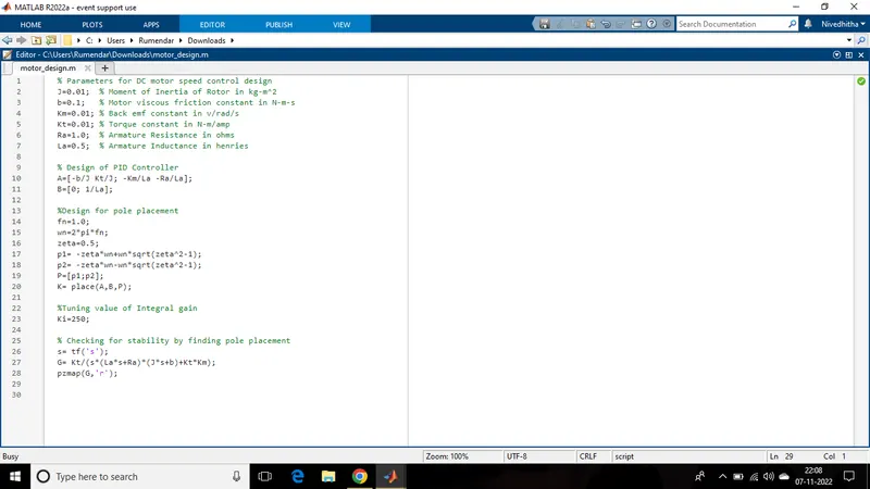
The matlab script file for DC Motor
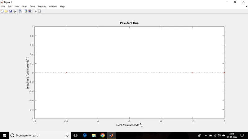
Here the poles of the system lies in left half plane. Thus the system become stable in nature.
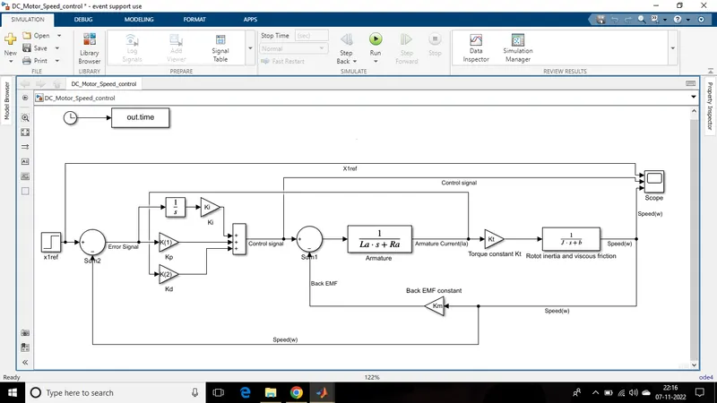
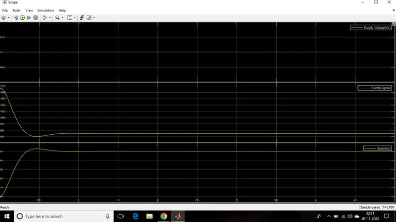
After implementing PID controller in DC motor dynamic system
Steady state error has been eliminated
There is max peak of overshoot is 5.25 and undershoot is 4.98
Rise time is 0.3 sec.
Settling time is 1.25 sec