Project - Speed Control of a Direct Current (DC) motor
OBJECTIVE:
In this project, a Simulink model for the DC motor will be first developed per the schematic shown in Figure 1.
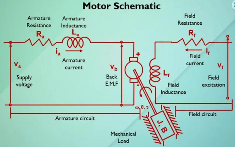
Use the Proportional, Integral, and Derivative (PID) control design knowledge gained in the training to design, develop and test a controller to maintain a desired speed for the motor.
Key Highlights:
Mathematical modeling from the first principles
Modeling an Electrical Engineering system
Simulink based modeling
Control law design and test
Stability of a dynamic system
Deliverables:
MATLAB script to define modeling and control design parameters
Simulink model to simulate and verify the design
Solution:
In this project, we are building a DC motor in two cases.
Case-1: DC motor without controller
Case-2: DC motor with the controller.
Firstly, we design a DC motor with Mathematical equations. Here I am taking the circuit diagram of a dc motor which is given in the project objective.
The Motor schematic diagram is shown below:
Modeling of a DC Machine:
What is a DC Motor?
A DC motor is an electrical machine that converts electrical energy into mechanical energy. In a DC motor, the input electrical energy is the direct current which is transformed into mechanical rotation.
Modeling of a DC Motor:
Modeling of a dc motor by using the below circuit model and taking the parameters as per the lecture.
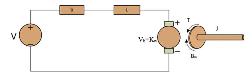
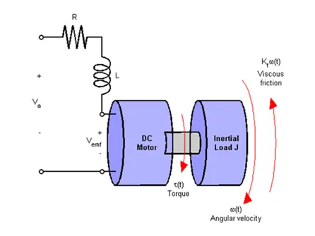
J = Moment of Inertia of Rotor.
B = Damping Coefficient.
R = Armature resistance
L = Armature Inductance
Vb = Back emf constant
KT = Motor Torque Constant
V = Supply Voltage
Motor Torque T = KT * I
Back EMF Vb = Kb * ω = Kb * dθ/dt
Finding equations, from the below figure:
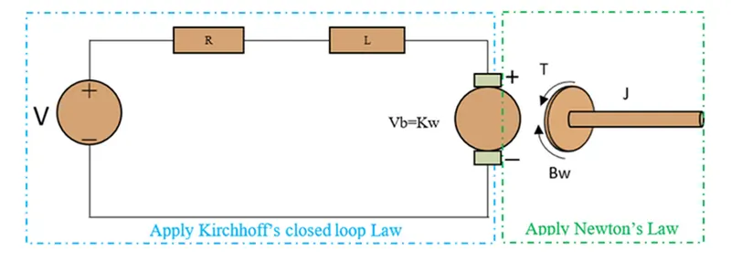
As per Kirchhoff’s Voltage Law
V = IR + L (di/dt) + Vb
L (di/dt) + IR = V - Kb (dθ/dt) ----equ-(a)
As per Newtons Law
J (d2θ/dt2) + B (dθ/dt) = KT * I ----equ-(b)
Converting the above equations to the S domain (Laplace Transform)
Laplace of equ – (a)
LsI(s) + RI(s) = V(s) - Kbsθ(s) ----equ-(c)
I(s) = V(s) - Kbsθ(s)/Ls + R ---- equ-(d)
Laplace of equ – (b)
Js2 θ(s) + Bs θ(s) = KT * I(s) ---equ-(e)
ωs = s θ(s) = KT * I(s)/Js+B ----equ-(f)
Substitute I(s) value in equ-(e)
Js2 θ(s) + Bs θ(s) = KT * I(s) ---equ-(e)
Js2 θ(s) + Bs θ(s) = KT * (V(s) – Kbsθ(s))/ (Ls + R) ---equ-(g)
s θ(s)[(Js+B) * (Ls+R)] = KTV(s) – KT * Kbsθ(s)
s θ(s)[(Js+B) * (Ls+R)] + KT * Kbsθ(s)= KTV(s)
s θ(s)[(Js+B) * (Ls+R) + (KT * Kb)]= KT V(s)
The transfer function of output angle θ(s) to the input angle V(s) is given by
Ga(s) = θ(s)/V(s) = KT / s[(Ls+R) * (Js+B) + (KT * Kb)] ----equ-(h)
The transfer function of the output angle ω(s) to the input angle V(s) is given by
Ga(s) = (s)/V(s) = KT / [(Ls+R) * (Js+B) + (KT * Kb)] ----equ-(i)
Case-1: DC motor without a controller.
By using the above transfer function equations, the DC motor is developed.
Simulink Model of DC Motor:
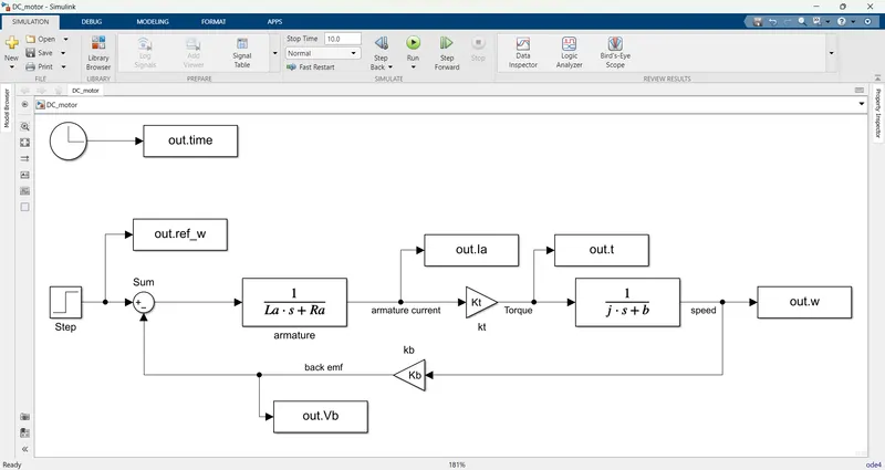
Blocks used in the simulation:
Step
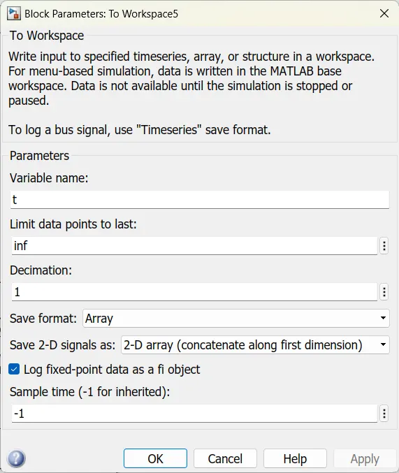
to workspace
sum
transfer function
gain
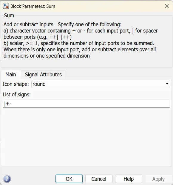
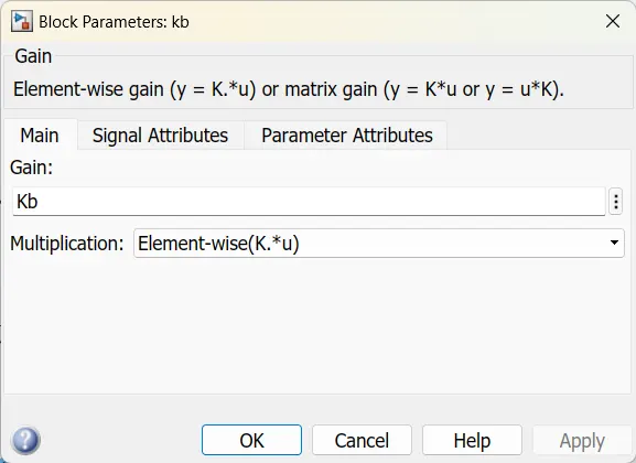
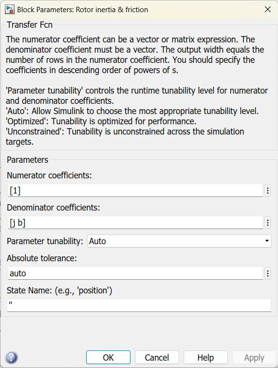
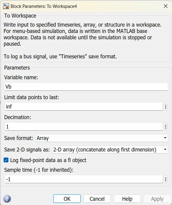
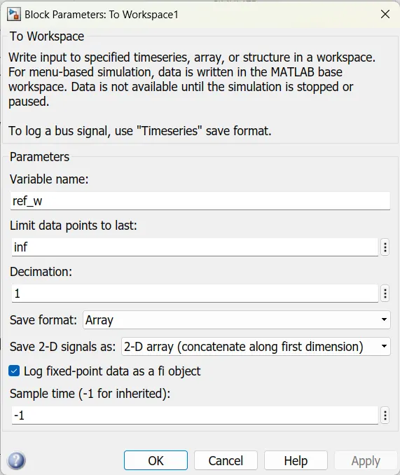
The properties of Each block are shown below:
Model building:
Firstly, we are taking a sum block with two input terminals one is positive for taking input from the constant or step block input as reference input. And another port is a negative port this port is connected to a feedback gain block output port. Which is the feedback signal taken from the speed (output of the second transfer function). Then the output of the sum block is given to a transfer function block which is calculating the La and Ra. Then the output of the transfer function block is multiplied with a gain block named Kt and here we can get the torque from the output of the gain block it is calculated with the second transfer function block and the output is speed. Then the speed is integrated with an integrator here the displacement is the output and it is given to a workspace block. By plotting the graph between the time vs speed, current, and voltage we can observe the system response.
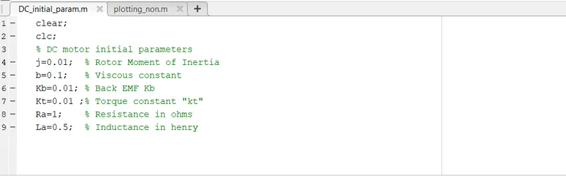
In the below figure we can see the DC MOTOR PARAMETERS in m-script:
M-script explanation for Initial values and plotting:
In the above script, we are defining the DC motor’s initial parameters to run the model and observe the response of the system.
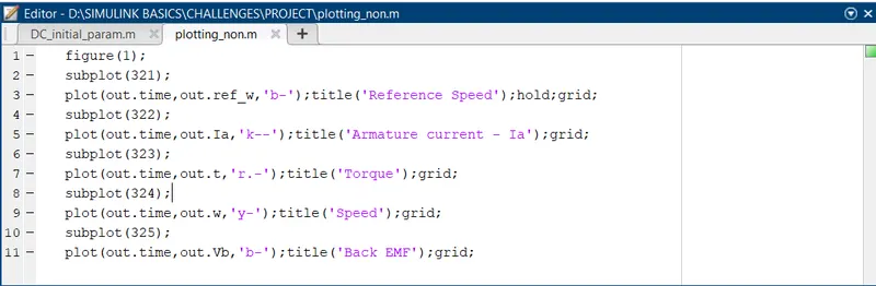
Plotting Script:
Result:
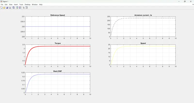
In the above plot, we can observe the response of the system without a controller.
Case-2: DC Motor with PID controller
In case 1, we developed a DC Motor without a controlling system.
Here we use a PID controller to control the motor.
Modeling of a DC Motor with PID controller
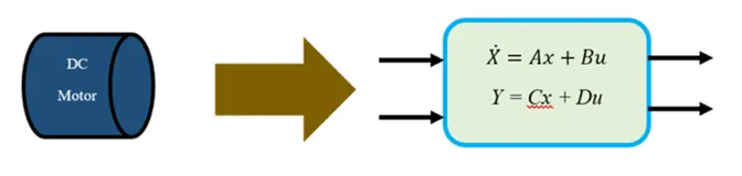
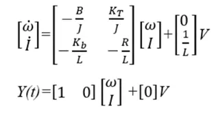
State Space equations for the DC Motor
State equations will be derived from equations (a) and (b)
dI/dt = - (R/L) I + (1/L) V – (Kb/L) d/dt
dI/dt = - (R/L) I + (1/L) V – (Kb/L) ω dI/dt
dω/dt= - (B/J) ω + (1/J) KTI
Y(t) = ω = d/dt
A state space representation of the DC motor from the above equations
Modeling of DC Motor with PID Controller:
What is PID Controller?
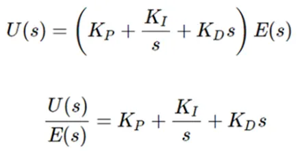
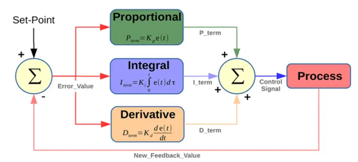
A proportional-integral-derivative controller (PID controller or three-term controller) is a control loop mechanism employing feedback that is widely used in industrial control systems and a variety of other applications requiring continuously modulated control. The proportional integral derivative controller produces an output, which is the combination of the outputs of proportional, integral, and derivative controllers. The feedback from the plant whichever is a controllable parameter is given as input to the PID controller and the processed error is minimized to get the desired output if tuning of the parameter is done optimally. The mathematically PID controller can be defined by the following equation where e(t) is the error signal with respect to time, Kp, Ki and KD are PID constants.

Apply Laplace transform on both sides.
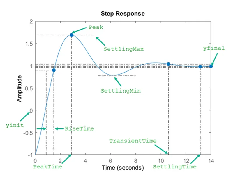
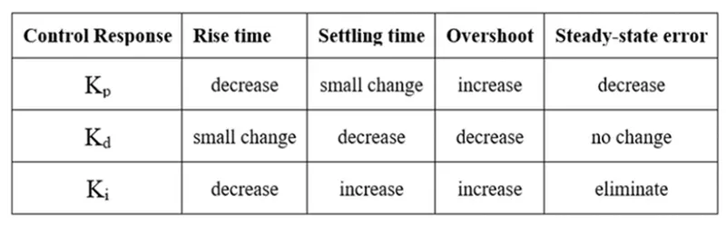
The parameter which is under control must have some properties or be free from some properties such as rise time, settling time, overshoot, and steady-state error. The impact of PID parameters on such properties can be found in the below table.
Rise Time:
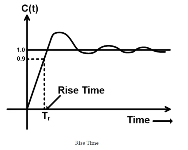
Rise time is defined as the time taken for a signal to cross from a specified low value to a specified high value. In analog and digital electronics, the specified lower value and specified higher value are 10% and 90% of the final or steady-state value. So, the rise time is typically defined as how long it takes for a signal to go from 10% to 90% of its final value.
Settling Time
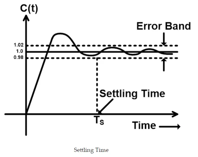
The settling time of a dynamic system is defined as the time required for the output to reach and steady within a given tolerance band. It is denoted as Ts. Settling time comprises propagation delay and time required to reach the region of its final value. It includes the time to recover the overload condition incorporated with slew and steady near to the tolerance band.
The tolerance band is the maximum allowable range in which the output can be settled. Generally, the tolerance bands are 2% or 5%.
Peak Over Shoot:

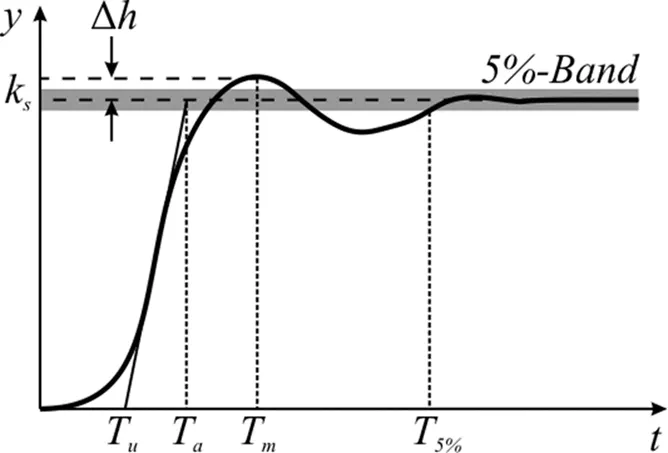
(MP) is defined as the deviation of the response at the peak time from the final value of the response. it is also called the maximum overshoot. We can write it as
Steady State Error:
Steady-state error is defined as the difference between the desired value and the actual value of a system output in the limit as time goes to infinity (i.e., when the response of the control system has reached steady-state).
Steady-state error is a property of the input/output response for a linear system. In general, a good control system will be one that has a low steady-state error.

Stability of the System:
A system is stable if every bounded input yields a bounded output. We call this statement the bounded-input, bounded-output (BIBO) definition of stability.
The stability of a linear closed loop system can be determined from the locations of the closed loop poles in the s-plane.
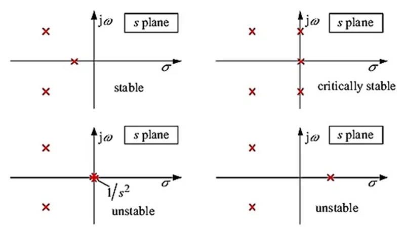
The location of the poles of the transfer function decides the stability of the system. This is shown in the above figure for critically stable, unstable, and stable systems.
For our case, the transfer function is determined from the constants of motor and state space equations,
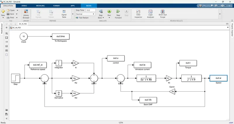
DC motor with PID controller simulation model shown below:
Blocks used in the simulation:
Step
clock
to workspace
sum
integrator
derivative
gain
transfer function
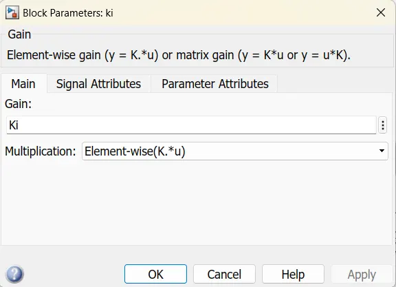
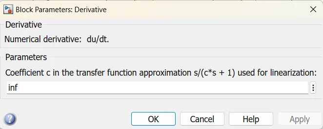
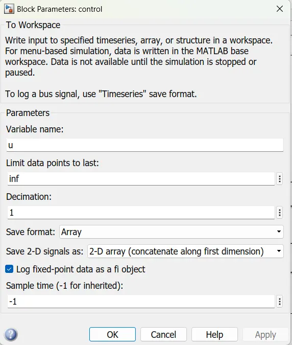
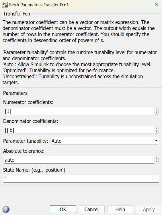
The properties of Each block are shown below:
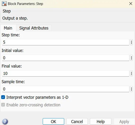
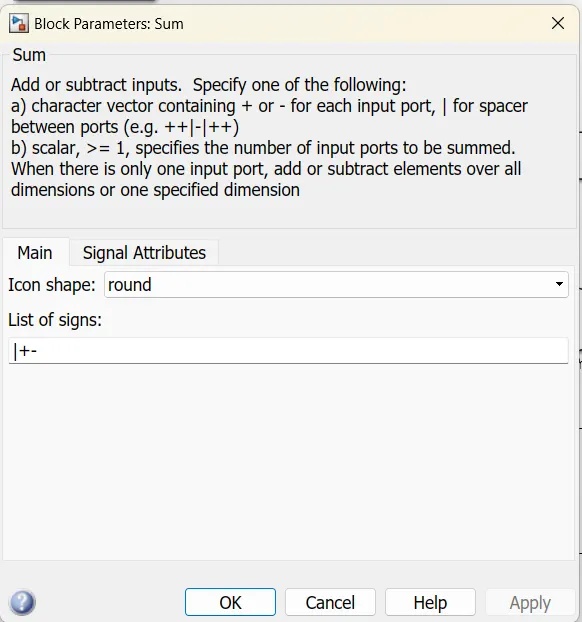
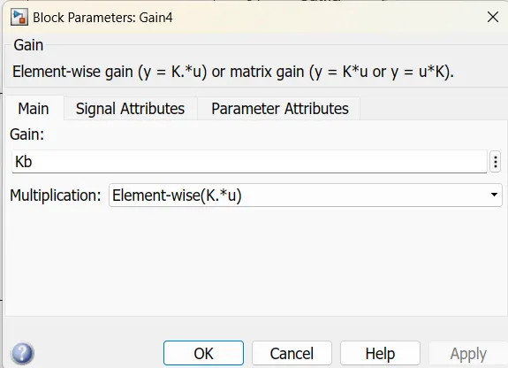
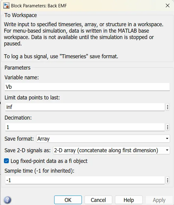
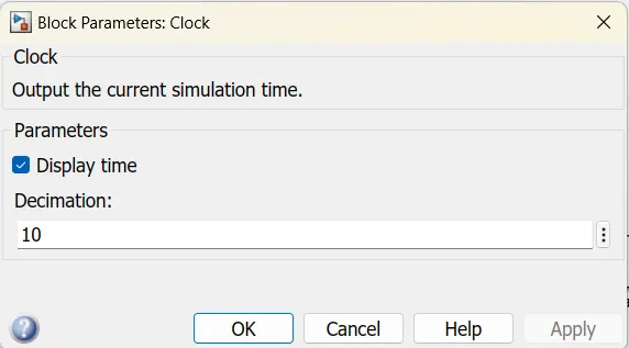
M-script for the model is shown below:
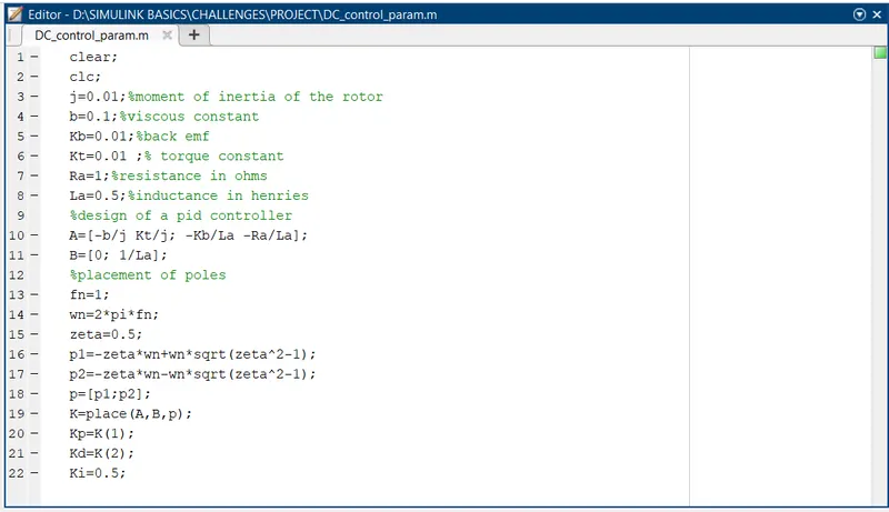
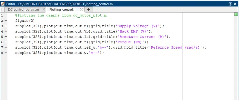
The plotting script is shown below:
Model explanation:
For building the DC motor with the PID controller simulation model we use the Simulink primitive blocks. Firstly, we took a clock block and a to workspace block that is connected to each other. Then for a reference speed, we took a step input block with a step size of 5 and a final value of 10. Then it was connected to a sum block which is having two input ports positive and negative. The positive input port has a step input and the negative port is connected between the integrator and to workspace named ‘w’. then the output of the sum block is given to a controller gain block named Kp. For the Integral Ki a gain block is used with initial conditions as zero. For the derivative gain, we are taking a derivative block connected to a gain block named Kd, and all the PID gains output is connected to a sum block with positive ports. Then its output is given to another sum block positive port and the negative port is connected to the back emf gain block. Ant its input is taken from the second transfer function output as a feedback signal. The second sum block output is given to a transfer function having impedance and resistance values and its output is multiplied with a gain block which is torque constant Kt. By multiplying the kt and transfer function we get Torque as output and it is given to another transfer function then the output is a speed and it is given to the workspace block. this simulation is run for 10 seconds and the system response is verified by plotting the graph between time vs speed and ref_speed.
M-script Explanation:
To run the model, we use a script file. In this script, we are defining the model parameters as taken in the lecture. For the PID controller design, we are taking the equations which are solved to develop the Simulink model. And here we are defining the matrices A and B. for the pole placement we take the fn as natural frequency. And wn is calculated for natural frequency in rad/sec. the zeta value is taken as 0.5. to calculate the poles, we use the below formulas: p1=-zeta*wn+wn*sqrt(zeta^2-1);
p2=-zeta*wn-wn*sqrt(zeta^2-1);
the by using the “place” command we place the poles in the plot. We define the PID values as Kp, Kd, and Ki. The transfer function is defined and poles are mapped for the given G1 transfer function.
After running the script successfully without errors for 10 seconds. We can observe the result in the workspace window and the poles are plotted in a new window.
Result:
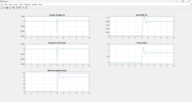
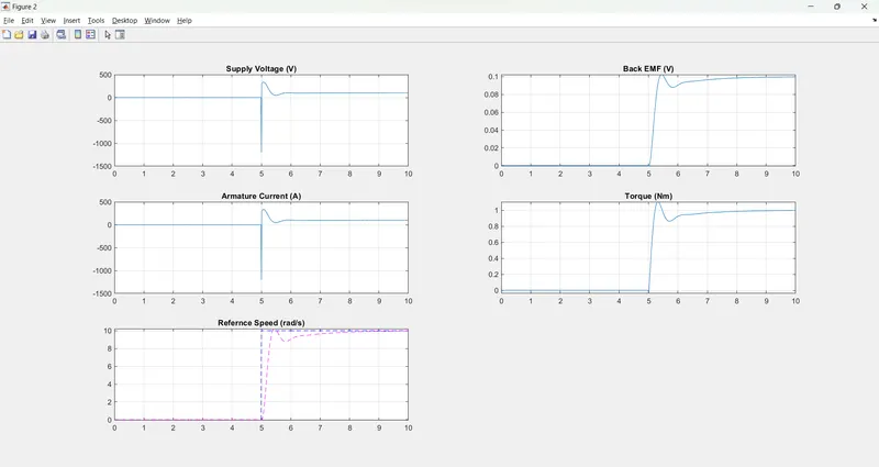
The simulation is run for 10 seconds and the settling time, overshoot, and steady-state error conditions are met.
Test-1: kp=38.3133, kd= -2.8584, Ki= 0.5000
The plot response with the above gain’s values is shown below.
Test-2: Kp=30, Kd=-1.5, Ki= 30
Test-3: Kp=30, Kd=-0.9, Ki= 60
The plot response with the above gain’s values is shown below.
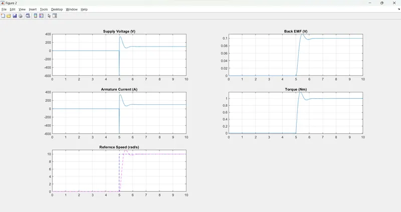
In the above plot, we can observe the reference speed plot. the speed is controlled by PID controller and matched with the reference wave. in this plot the steady state error, overshoot, and rise time conditions are satisfied. the best response of the overall three test conditions is test 3.
Conclusion:
The dc motor without control and with the controller is designed and its plot response is observed. The controller is tested under various values of controller gains. The best response is test-3 and it satisfied the conditions.