Project - Speed Control of a Direct Current (DC) motor

SPEED CONTROL OF A DIRECT CURRENT DC MOTOR

A PROJECT

OBJECTIVE

For the function of designing and developing the PID controller for a DC motor, an approximate Matlab programme was used. From there, a set of equations was developed using the Simulink model, and the

AIM

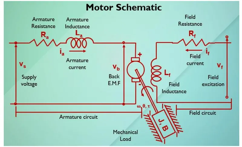
Using a PID controller, a dc motor's target speed may be designed, developed, and maintained with some gains like Kp, Kd, and Ki. When designing a PID, the estimated field excitation is used to maintain the desired load voltage. Kirchhoff law is then used to compute the armature resistance (Ra), armature inductance (La), and moment of inertia (J). The motor schematic shown in figure1.

PID CONTROLLER

One type of feedback controller is PID. The past, present, and future errors are used by this straightforward sort of controller, and it is these fundamental qualities that you require to address most control problems. Because of this, PID is the most often used type of feedback control in a variety of physical applications.

PARAMETERS USED:

J - Moment of inertia of rotor - 0.01 Kg m²

B - Motor viscous friction constant - 0.1 Nms.

Km – Back emf constant - 0.01 radians/sec

Kt - Motor torque constant – 0.01 Nm/Ampere

Ra – Armature resistance – 1.0 Ohm

La – Armature inductance – 0.5 Henry

ASPECTS OF THE SYSTEM

A DC motor's torque is often inversely correlated with its armature current and magnetic field intensity. For the sake of this illustration, we will assume that the magnetic field is constant and that the motor torque is proportional to simply the armature current (I) by a constant factor K_t, as indicated in the equation below. A motor like this is referred to as armature controlled.

The back emf, , is proportional to the angular velocity of the shaft by a constant factor

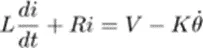
Since the motor torque and back emf constants are equivalent in SI units, we shall use as a single unit to denote both constants. The following governing equations, which are based on Kirchhoff's voltage law and Newton's second law, may be derived from the preceding graphic.

TRANSFER FUNCTION

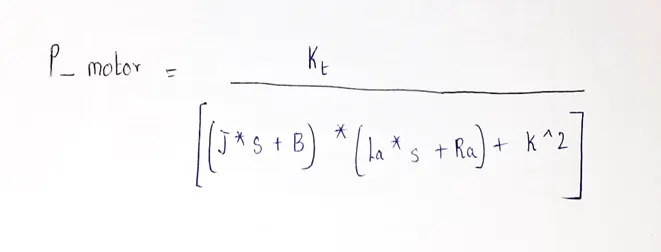
Applying the Laplace transform, the above modelling equations can be expressed in terms of the Laplace variable s.

STATE SPACE FUNCTION

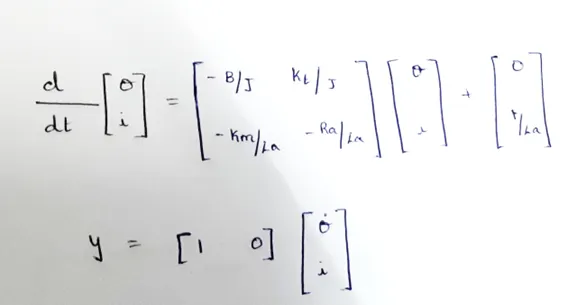
The governing equations above may be represented in state-space form by using the electric current and rotational speed as the state variables. Once more, the rotational speed is selected as the output and the armature voltage is used as the input.

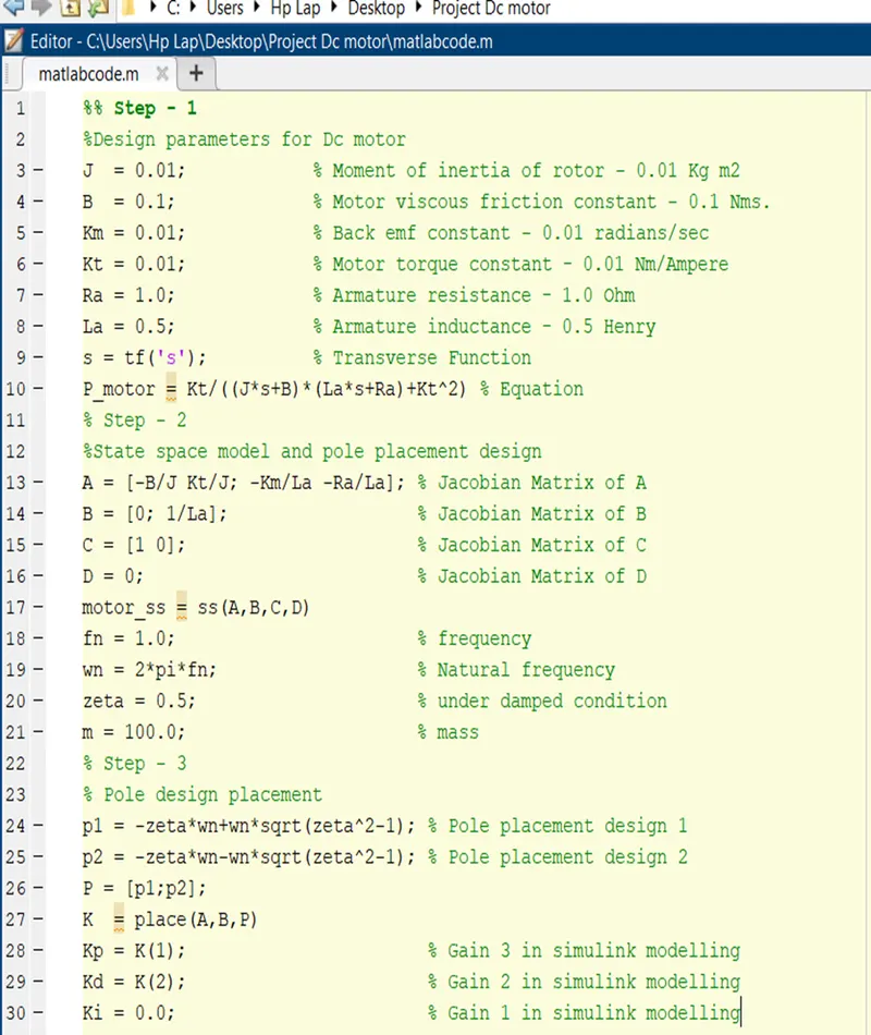
MATLAB CODE 1

%% Step - 1

%Design parameters for Dc motor

J = 0.01; %Moment of inertia of rotor - 0.0Kg m2

B = 0.1; % Motor viscous friction constant - 0.1 Nms.

Km = 0.01; % Back emf constant - 0.01 radians/sec

Kt = 0.01; % Motor torque constant – 0.01 Nm/Ampere

Ra = 1.0; % Armature resistance – 1.0 Ohm

La = 0.5; % Armature inductance – 0.5 Henry

s = tf('s'); % Transverse Function

P_ Motor = Kt/((J*s+B)*(La*s+Ra)+Kt^2)

% %Step - 2

%State space model and pole placement design

A = [-B/J Kt/J; -Km/La -Ra/La]; % Jacobian Matrix of A

B = [0; 1/La]; % Jacobian Matrix of B

C = [1 0]; % Jacobian Matrix of C

D = 0; % Jacobian Matrix of D

motor_ss = ss(A, B, C, D)

fn = 1.0; % frequency

wn = 2*pi*fn; % Natural frequency

zeta = 0.5; % under damped condition

m = 100.0; % mass

%% Step - 3

% Pole design placement

p1 = -zeta*wn+ wn*sqrt(zeta^2-1); % Pole placement design 1

p2 = -zeta*wn-wn*sqrt(zeta^2-1); % Pole placement design 2

P = [p1; p2];

K = place(A,B,P)

Kp = K(1); % Gain 3 in Simulink modelling

Kd = K (2); % Gain 2 in Simulink modelling

Ki = 0.0; % Gain 1 in Simulink modelling

MATLAB CODE 2

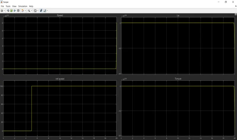
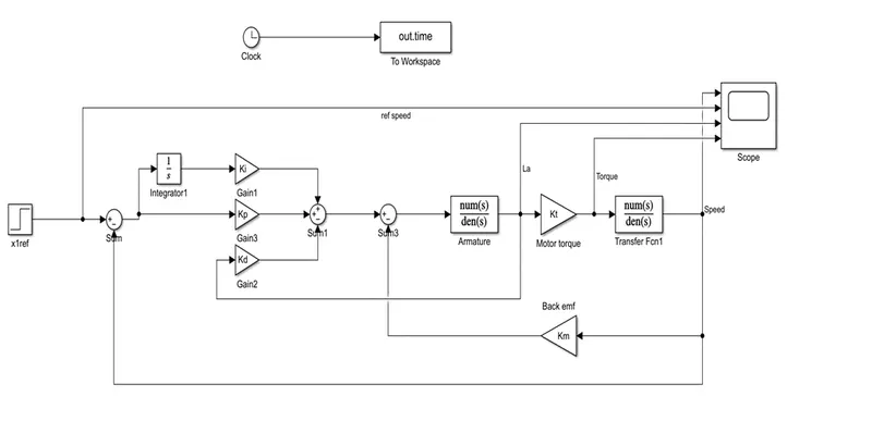
SIMULINK MODEL

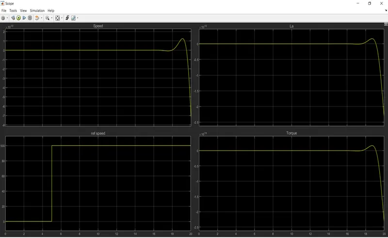
SIMULINK MODEL 1 WITH GIVEN GAIN VALUES:-

Kp = 38.3.

Kd = -2.85.

Ki = 0.0.

SIMULINK MODEL 2 WITH DIFFERENT GAIN VALUES: -

Kp = 50.

Kd = 25.

Ki = 10.

.

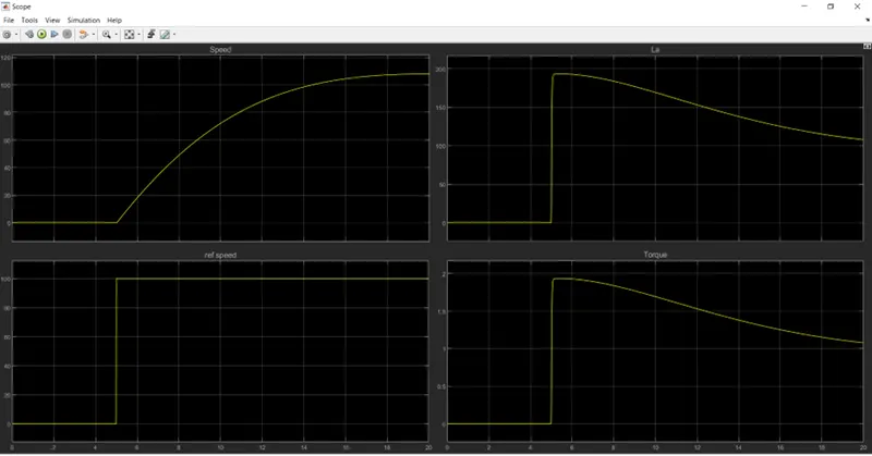
SIMULINK MODEL 3 WITH DIFFERENT GAIN VALUES: -

Kp = 100.

Kd = 150.

Ki = 50.