Project 1

DEALS WITH THE DEVELOPMENT OF FORWARD DEVELOPMENT OF A FORWARD ENERGY BASED FUEL CONSUMPTION MODEL OF A CONVENTIONAL VECHILE

OBJECTIVE

For the goal of estimating the driver, controller, and powertrain, construct a fuel-based conventional vehicle model utilising the UDDS and HWFET drive cycle, and plot the engine speed, torque, transmission, differential, wheel, and distance travelled.

AIM

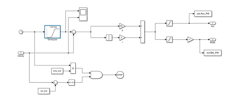
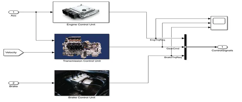
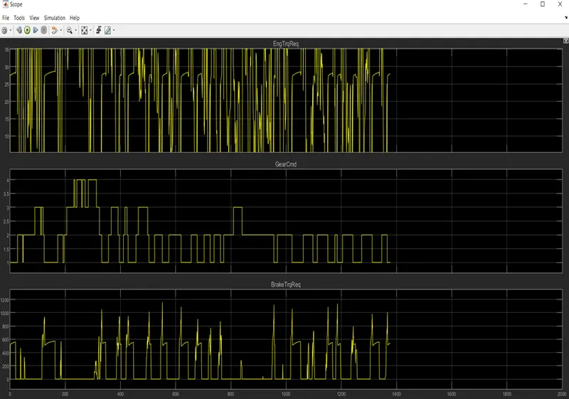
The primary objective of this project is to get experience with the modelling process, including developing MATLAB scripts, modelling in Simulink, evaluating data, and producing graphs. This idea considers a typical midsize automobile with a 1.9L engine and a 4-speed automatic transmission. The updating the information has the capacity to replicate the car on several driving cycles, including UDDS, HWFET, FTP, NEDC, etc. It is modelled using a "Driver" block, a simple PI controller that creates pedal outputs for the acceleration and brake that correspond to the desired and actual vehicle speeds. The "Controller" block, which stands in for the electronic control systems, is the vehicle's central processing unit. It produces the desired engine torque, transmission gear, and brake torque based on the inputs from the driver.

CONVENTIONAL VEHICLES

The combustion of a fuel takes place with the help of an oxidizer (often air) in a combustion chamber that is a crucial component of the working fluid flow circuit in an internal combustion engine (ICE or IC engine). In an internal combustion engine, a component is subjected to direct force as a result of the expansion of the high-temperature and high-pressure gases generated during combustion. Typically, the force is applied to a rotor (Wankel engine), turbine blades (gas turbine), pistons (piston engine), or a nozzle (jet engine). The component is propelled across a distance by this force, which converts chemical energy into kinetic energy that is then utilised to move or power whatever the engine is connected to. . For situations where the weight or size of an engine was more crucial, this took the role of the external combustion engine. Despite having several fixed uses, ICEs are mostly employed in mobile applications and serve as the main power source for cars, boats, and other moving objects. Hydrocarbon-based fuels like ethanol, natural gas, gasoline, or diesel fuel are frequently used to power ICEs. Compression ignition (CI) engines utilise biodiesel as a fuel, whereas spark ignition (SI) engines use bioethanol or ETBE (ethyl tert-butyl ether), which is made from bioethanol. Rudolf Diesel, the creator of the diesel engine, was using peanut oil to power his machines as early as 1900. Frequently, fossil fuels and renewable energy are combined. Rarely used hydrogen can be produced using fossil fuels or clean energy sources.

This project demonstrates how to compute the emissions and fuel efficiency for a typical car with a 1.9-L engine on the city and highway. Installed for this project's operation are UDDS and highway (HWFET) driving cycles.

This project shows how to calculate the city and highway fuel economy and the emissions for a conventional vehicle with a 1.9-L engine. To run this project with UDDS and the highway (HWFET) drive cycles are installed.

SIMULINK BLOCK

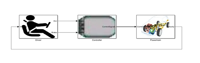
DRIVER

A driver is a piece of functionality that permits communication between a clutch, a brake, and a speed. To manage the many installed hardware components like pedals, steering, etc., each IC engine has a number of drivers. Without these drivers, the hardware and software may not operate correctly or perhaps at all in some circumstances. Drivers are files that an engine uses to communicate requests to hardware or programmes. The drivers convert engine communications into a language that the hardware or application can comprehend. Not every device driver interacts with the device in real time. There may be several drivers stacked in different ways to facilitate communication in various circumstances. Direct communication between the drivers at each end of the road and the vehicle's operational components will take place. The drivers in between change the communication's forms so that the machine can understand them.

CONTROLLER

Devices called controllers are used to control how an electric motor operates. Motor controllers are often utilised in conjunction with switchboards or VFDs to regulate the functioning of the primary mover in artificial lift applications. A manual or automatic method for starting and halting the motor, choosing forward or backward rotation, accelerating or decelerating, and managing other operating parameters is frequently included in controllers. Additionally, by controlling or restricting torque and guarding against overloads and malfunctions, motor controllers can offer protection for the artificial lift system. Many controllers provide extra features like data logging and collecting in addition to application-specific control logic.

POWERTRAIN

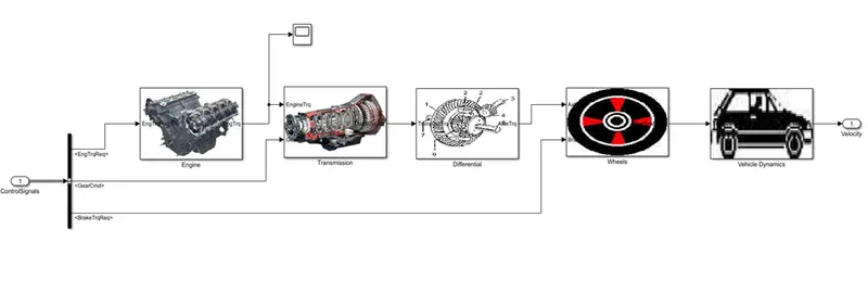
The collection of all the parts that propels your car forward is called the powertrain. The engine of your automobile generates power, which the powertrain then transfers to the wheels on the ground. Engine, gearbox, wheels, vehicle dynamics, and differential are the main parts of a powertrain. Let's examine each in turn:

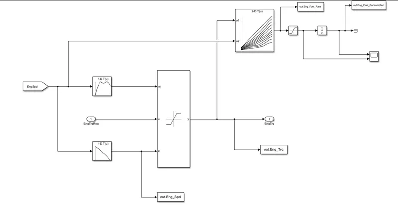
Engine: The engine is the driving force behind your car and serves as its heart. The components of an engine are pistons that oscillate inside of cylinders and a crankshaft that converts the oscillating action into a rotational motion.

Transmission: A transmission is a basic component in your car that makes sure the proper amount of power is transmitted to the wheels. Like a car's gearbox, the transmission takes the power from the engine and adjusts it according to driving conditions, ultimately transferring it to the wheels.

Wheels: A drivewheel is a motor vehicle's wheel that transfers force by converting torque into tractive force from the tyres to the road, which moves the vehicle. The vehicle moves forward or backward as a result of the powertrain's ability to supply enough torque to the wheel to overcome stationary forces. While a four-wheel drive vehicle has four driven wheels, a two-wheel drive vehicle only has two driven wheels, often both in the front or rear.

Differential: One component of the rear axle is a differential. It enables the back wheels to rotate at various speeds. The differential, for instance, is crucial when rounding a bend since the outside wheel must turn more quickly than the inner wheel. Your car cannot go ahead without a functioning powerplant; thus it is essential. In summary, it is a collection of components that produce, transform, and use energy to propel your vehicle forward.

Vehicle Dynamics: Tire properties are intimately correlated with vehicle dynamics. The angle between the direction of the tire's heading and travel direction is known as the tyre slip angle because it occurs when the vehicle's lateral force is applied to its four tyres, causing them to side-slide.

VEHICLE PERFORMANCE

The evaluation of a vehicle's motion is known as vehicle performance. Any vehicle's motion is dependent on all the forces and moments acting on it. The majority of these forces and moments are brought on by the interaction of the vehicle with the surrounding medium(s), including air or water (e.g., fluid static and dynamic forces), gravitational attraction (gravity forces), the Earth's surface (support, ground, or landing gear forces), and on-board energy-consumption components like rocket, turbojet, piston engine, and propellers (propulsion forces). Consequently, it is vital to research and, in some manner, describe these interacting factors in order to completely comprehend the performance issue.

CONVENTIONAL POWERTRAIN EFFICENCY

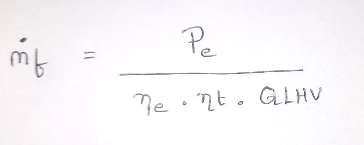
For conventional Ic engine vehicle the wheels power is supplied by engine through transmission drivertrain efficiency

Were

mf = mass flow rate in [kg]

pe = Power of engine

pt = Power of transmission

nt = efficiency of transmission

DRIVER BLOCK

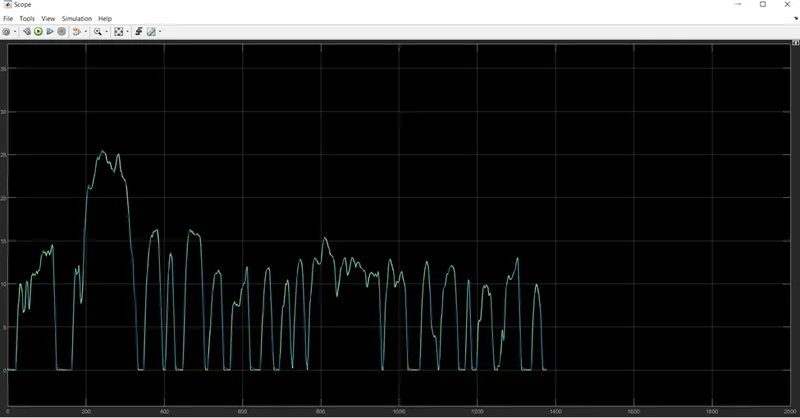
DRIVER BLOCK OUTPUT

CONTROLLER BLOCK

CONTROLLER BLOCK OUTPUT

VEHICLE DYNAMICS

ENGINE BLOCK

ENGINE OUTPUT

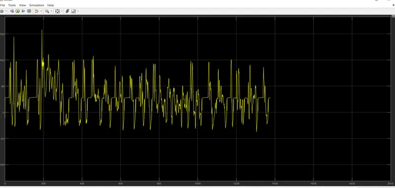
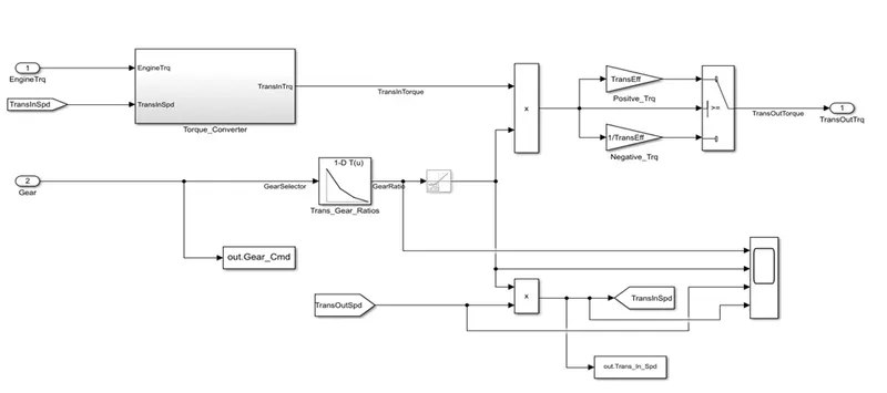
TRANSMISSION BLOCK

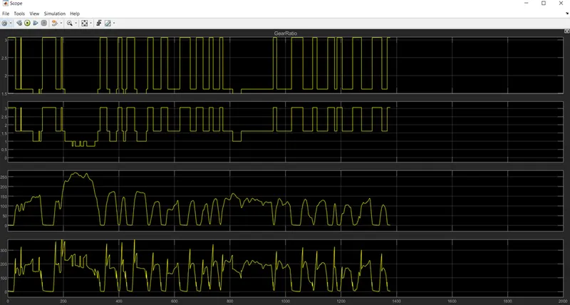
TRANSMISSION BLOCK OUTPUT

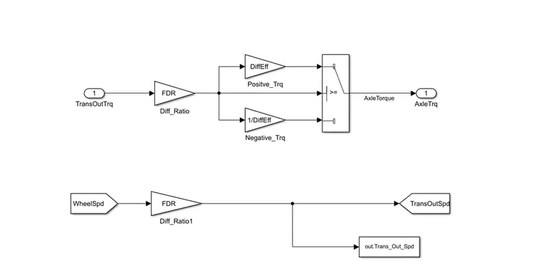
DIFFERENTIAL BLOCK

WHEELS BLOCK

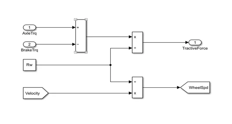
VEHICLE DYNAMICS

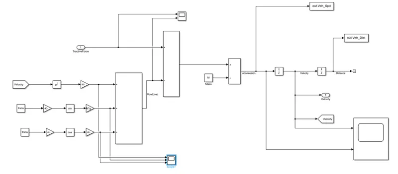
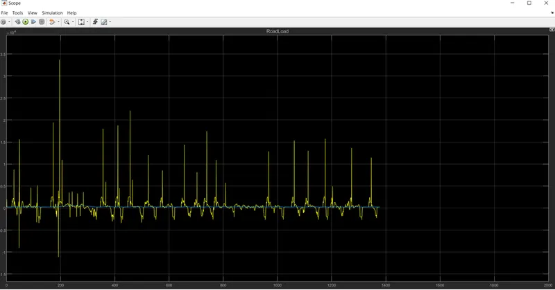
VEHICLE DYNAMICS - ROADLOAD

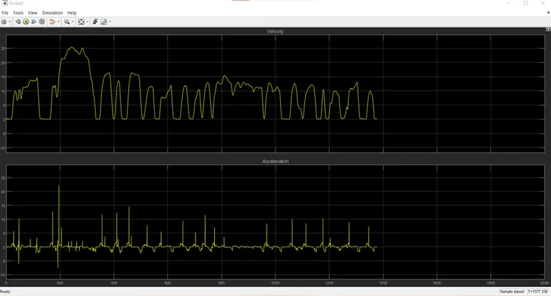
VEHICLE DYNAMICS – VELOCITY AND ACCELERATION

MATLAB CODE

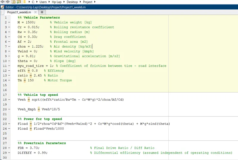
VEHICLE PARAMETERS

M = 1500; % Vehicle weight [kg]

Cr = 0.015; % Rolling resistance coefficient

Rw = 0.35; % Rolling radius [m]

Cd = 0.33; % Drag coefficient

Af = 2; % Frontal area [m2]

rhoa = 1.225; % Air density [kg/m3]

Vwind = 0; % Wind velocity [kmph]

g = 9.81; % Gravitational acceleration [m/s2]

theta = 0; % Slope [deg]

myu_road_tire = 1; % Coefficient of friction between tire - road interface

efft = 0.8 % Effiency

ratio = 2.45 % Ratio

Tm = 150 % Motor Torque

Vehicle top speed

Vveh = sqrt((efft*ratio/Rw*Tm - Cr*M*g)*2/rhoa/Af/Cd)

Vveh_Kmph = Vveh*18/5

Power for top speed

Fload = 1/2*rhoa*Cd*Af*(Vveh+Vwind)^2 + Cr*M*g*cosd(theta) + M*g*sind(theta)

Pload = Fload*Vveh/1000

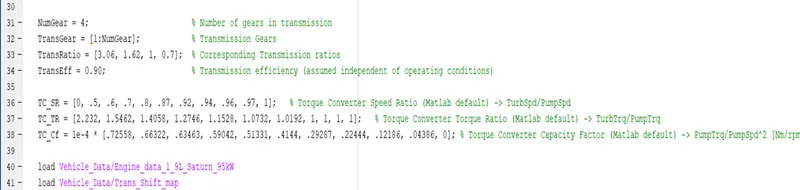
Powertrain Parameters

FDR = 3.73; % Final Drive Ratio / Diff Ratio

DiffEff = 0.99; % Differential efficiency (assumed independent of operating conditions)

NumGear = 4; % Number of gears in transmission

TransGear = [1:NumGear]; % Transmission Gears

TransRatio = [3.06, 1.62, 1, 0.7]; % Corresponding Transmission ratios

TransEff = 0.90; % Transmission efficiency (assumed independent of operating conditions)

TC_SR = [0, .5, .6, .7, .8, .87, .92, .94, .96, .97, 1]; % Torque Converter Speed Ratio (Matlab default) -> TurbSpd/PumpSpd

TC_TR = [2.232, 1.5462, 1.4058, 1.2746, 1.1528, 1.0732, 1.0192, 1, 1, 1, 1]; % Torque Converter Torque Ratio (Matlab default) -> TurbTrq/PumpTrq

TC_Cf = 1e-4 * [.72558, .66322, .63463, .59042, .51331, .4144, .29287, .22444, .12186, .04386, 0]; % Torque Converter Capacity Factor (Matlab default) -> PumpTrq/PumpSpd^2 [Nm/rpm^2]

load Vehicle_Data/Engine_data_1_9L_Saturn_95kW

load Vehicle_Data/Trans_Shift_map

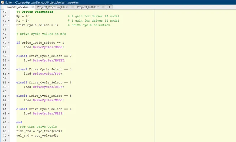
Driver Parameters

Kp = 10; % P gain for driver PI model

Ki = 1; % I gain for driver PI model

Drive_Cycle_Select = 1; % Drive cycle selection

Drive cycle values in m/s

if Drive_Cycle_Select == 1

load DriveCycles/UDDS;

elseif Drive_Cycle_Select == 2

load DriveCycles/HWFET;

elseif Drive_Cycle_Select == 3

load DriveCycles/FTP;

elseif Drive_Cycle_Select == 4

load DriveCycles/US06;

elseif Drive_Cycle_Select == 5

load DriveCycles/NEDC;

elseif Drive_Cycle_Select == 6

load DriveCycles/WLTP;

end

% For UDDS Drive Cycle installed in workspace
time_end = cyc_time(end);
vel_end = cyc_vel(end);

% For HWFET Drive Cycle installed in workspace
time_end1 = cyc_time1;
vel_end1 = cyc_vel1

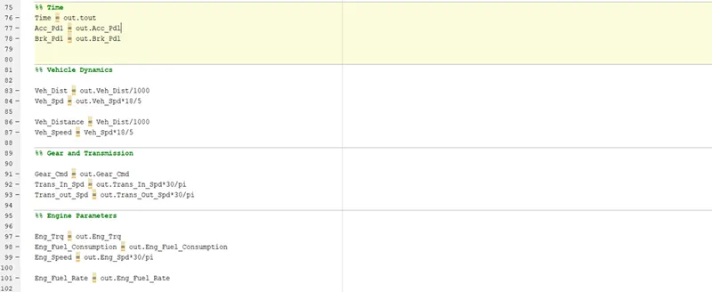
Time

Time = out.tout

Acc_Pd1 = out.Acc_Pdl

Brk_Pd1 = out.Brk_Pdl

Vehicle Dynamics

Veh_Dist = out.Veh_Dist/1000

Veh_Spd = out.Veh_Spd*18/5

Veh_Distance = Veh_Dist/1000

Veh_Speed = Veh_Spd*18/5

Gear and Transmission

Gear_Cmd = out.Gear_Cmd

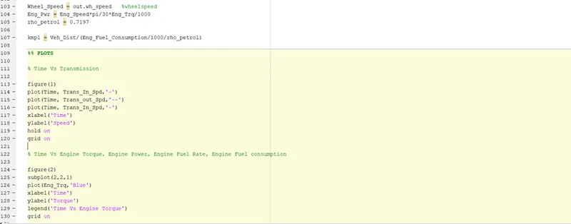
Trans_In_Spd = out.Trans_In_Spd*30/pi

Trans_out_Spd = out.Trans_Out_Spd*30/pi

Engine Parameters

Eng_Trq = out.Eng_Trq

Eng_Fuel_Consumption = out.Eng_Fuel_Consumption

Eng_Speed = out.Eng_Spd*30/pi

Eng_Fuel_Rate = out.Eng_Fuel_Rate

Wheel_Speed = out.wh_speed %wheelspeed

Eng_Pwr = Eng_Speed*pi/30*Eng_Trq/1000

rho_petrol = 0.7197

kmpl = Veh_Dist/(Eng_Fuel_Consumption/1000/rho_petrol)

PLOTS

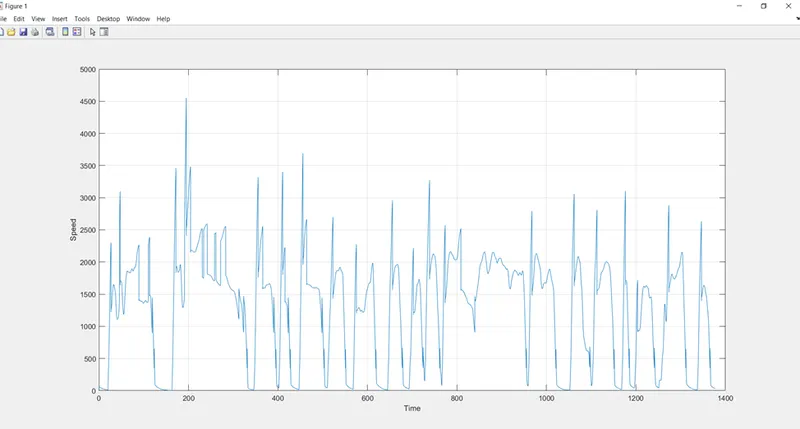
Time Vs Transmission

figure(1)

plot(Time, Trans_In_Spd,'-')

plot(Time, Trans_out_Spd,'--')

plot(Time, Trans_In_Spd,'-')

xlabel('Time')

ylabel('Speed')

hold on

grid on

figure(1)

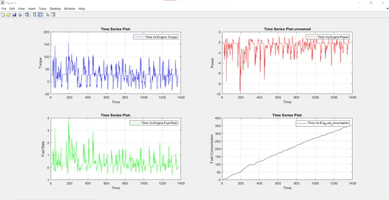
Time Vs Engine Torque, Engine Power, Engine Fuel Rate, Engine Fuel consumption

figure(2)

subplot(2,2,1)

plot(Eng_Trq,'Blue')

xlabel('Time')

ylabel('Torque')

legend('Time Vs Engine Torque')

grid on

subplot(2,2,2)

plot(Eng_Pwr,'Red')

xlabel('Time')

ylabel('Power')

legend('Time Vs Engine Power')

grid on

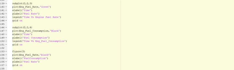
subplot(2,2,3)

plot(Eng_Fuel_Rate,'Green')

xlabel('Time')

ylabel('Fuel Rate')

legend('Time Vs Engine Fuel Rate')

grid on

subplot(2,2,4)

plot(Eng_Fuel_Consumption,'Black')

xlabel('Time')

ylabel('Fuel Consumption')

legend('Time Vs Eng_Fuel_Consumption')

grid on

figure(2)

UDDS DRIVE CYCLE

figure(2)

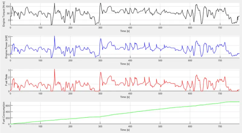
HWFET DRIVE CYCLE

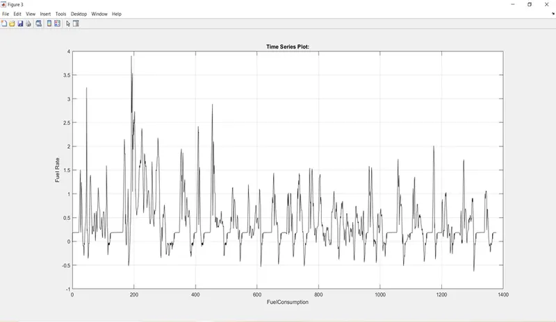
FUEL CONSUMPTION VS FUEL RATE

figure(3)

plot(Eng_Fuel_Rate,'black')

xlabel('FuelConsumption')

ylabel('Fuel Rate')

grid on

figure(3)

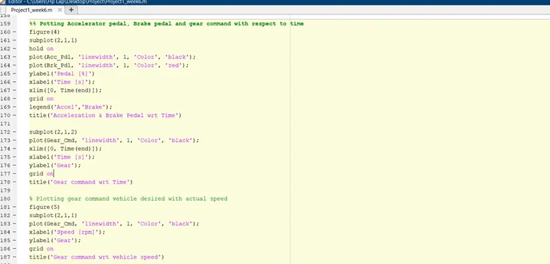
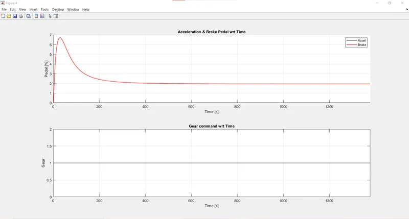
Potting Accelerator pedal, Brake pedal and gear command with respect to time

figure(4)

subplot(2,1,1)

hold on

plot(Acc_Pdl, 'linewidth', 1, 'Color', 'black');

plot(Brk_Pdl, 'linewidth', 1, 'Color', 'red');

ylabel('Pedal [%]')

xlabel('Time [s]');

xlim([0, Time(end)]);

grid on

legend('Accel','Brake');

title('Acceleration & Brake Pedal wrt Time')

subplot(2,1,2)

plot(Gear_Cmd, 'linewidth', 1, 'Color', 'black');

xlim([0, Time(end)]);

xlabel('Time [s]');

ylabel('Gear');

grid on

title('Gear command wrt Time')

figure4

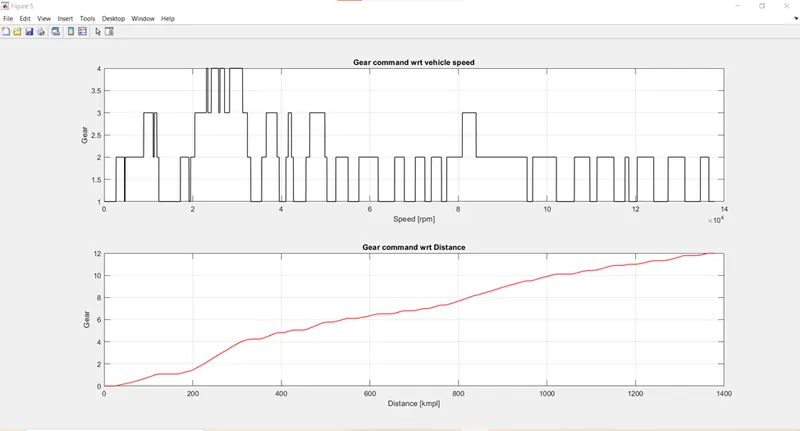
Plotting gear command vehicle desired with actual speed

figure(5)

subplot(2,1,1)

plot(Gear_Cmd, 'linewidth', 1, 'Color', 'black');

xlabel('Speed [rpm]');

ylabel('Gear');

grid on

title('Gear command wrt vehicle speed')

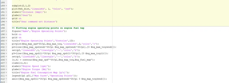
figure(5)

subplot(2,1,2)

plot(Veh_Dist,'linewidth', 1, 'Color', 'red');

xlabel('Distance [kmpl]');

ylabel('Gear');

grid on

title('Gear command wrt Distance')

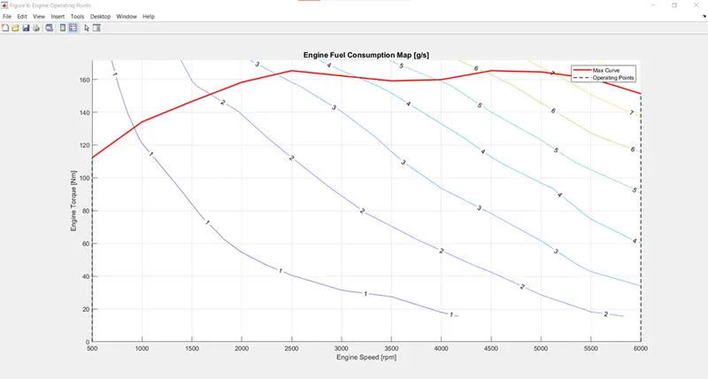
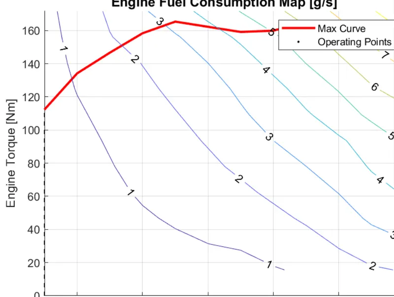
Plotting engine operating points on engine fuel map

figure('Name','Engine Operating Points');

hold on

grid on

title('Engine Operating Points','fontsize',12);

p1=plot(Eng_map_spd*30/pi,Eng_max_trq,'linewidth',2,'color','r');

p2=line([Eng_map_spd(end)*30/pi Eng_map_spd(end)*30/pi],[0 Eng_max_trq(end)]);

set(p2,'linewidth',1,'linestyle','--','color','k');

p3=line([Eng_map_spd(1)*30/pi Eng_map_spd(1)*30/pi],[0 Eng_max_trq(1)]);

set(p3,'linewidth',1,'linestyle','--','color','k');

[c,h] = contour(Eng_map_spd'*30/pi,Eng_map_trq,Eng_fuel_map');

clabel(c,h);

xlabel('Engine Speed [rpm]');

ylabel('Engine Torque [Nm]');

title('Engine Fuel Consumption Map [g/s]');

legend([p1 p3],{'Max Curve','Operating Points'});

axis([Eng_map_spd(1)*30/pi Eng_map_spd(end)*30/pi 0 Eng_map_trq(end)]);

figure(6)

UDDS DRIVE CYCLE

figure(6)

HWFET DRIVE CYCLE

MATLAB CODE